MATLAB程序设计：牛顿法求解非线性方程实例‌

1 牛顿迭代法

牛顿迭代法实质上是一种线性化方法，其基本思想是将非线性方程 $f(x)=0$ 逐步归结为某种线性方程来求解。

1.1 牛顿法

牛顿迭代法又称切线法，是一种有特色的求根方法。用牛顿迭代法求 $f(x)=0$ 的单根 $x^{*}$ 的主要步骤：

（1）Newton法的迭代公式

$x_{k+1}= x_{k}-\frac{f(x_{k})}{f'(x_{k}) } ，k=0,1,2,...$

（2）以 $x^{*}$ 附近的某一个值 $x_0$ 为迭代初值，代入迭代公式，反复迭代，得到序列 $x_1, x_2, x_3,...$

（3）若序列收敛，则必收敛于精确根 $x^{*}$ ，即 $\lim_{k\to\infty } x_k =x^*$ 。

牛顿法有显然的几何意义，方程 $f(x)=0$ 的根 $x^{*}$ 可解释为曲线与轴交点的横坐标。设 $x_k$ 是根 $x^{*}$ 的某个近似值，过曲线 $y=f(x)$ 上横坐标为 $x_k$ 的点 $P_k(x_k, y_k)$ 引切线，并将该切线与 $x$ 轴交点的横坐标 $x_{k+1}$ 作为 $x^{*}$ 的新的近似值。

牛顿法初值的选择：若 $f(x)$ 在 $[a,b]$ 上连续，存在2阶导数，且满足下列条件：

（1） $f(a)f(b)<0$ ；

（2） $f'(x)$ 在 $(a,b)$ 内不变号，且 $f'(x)\neq 0$ ；

（3） $f''(x)$ 在 $(a,b)$ 内不变号，且 $f''(x)\neq 0$ ；

（4） $\frac{\vert f(a) \vert }{\vert f'(a) \vert } \leq b-a$ ，且 $\frac{\vert f(b) \vert }{\vert f'(b) \vert } \leq b-a$ ；

则对任意的初值 $x_0\in [a,b]$ ，牛顿迭代序列收敛于 $f(x)=0$ 在 $[a,b]$ 内的唯一根。

牛顿的优缺点：牛顿法是目前求解非线性方程（组）的主要方法，至少二阶局部收敛，收敛速度较快，特别是当迭代初值充分靠近精确解时。对重根收敛速度较慢（线性收敛），对初值的选取很敏感，要求初值相当接近真解，需要求导数。

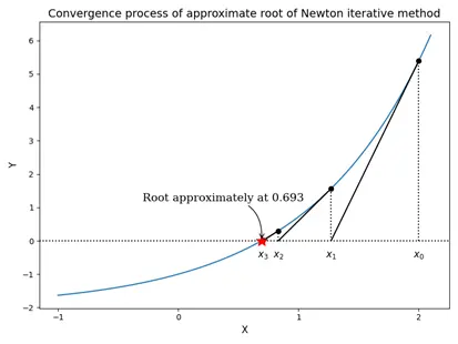
图1 牛顿法迭代收敛过程的几何意义

1.2 哈利牛顿法

哈利法（Halley）可用于加速牛顿法收敛，哈利迭代公式：

$x_{k+1}= x_{k}-\frac{f(x_{k})}{f'(x_{k}) } \left(1-\frac{f(x_k)f''(x_k)}{2(f'(x_k))^2} \right)^{-1}，k=0,1,2,...$

哈利法在单根情况下可达到三阶收敛。

1.3 简化牛顿法

将牛顿法的迭代公式改为

$x_{k+1}=x_k-\lambda f(x_k)，k=0,1,2,...$

为保证收敛，系数 $\lambda$ 只需满足 $0<\lambda <\frac{2}{f'(x_k)}$ 即可。如果 $\lambda$ 取常数 $\frac{1}{f'(x_0)}$ ，则称为简化牛顿法，也称平行弦法。

简化牛顿法线性收敛。

1.4 牛顿下山法

牛顿法的收敛性依赖初值 $x_0$ 的选取，如果 $x_0$ 偏离所求根 $x^*$ 较远，则牛顿法可能发散。牛顿下山法，引入下山因子 $\lambda$ ，保证函数值稳定下降的同时，加速收敛速度。

牛顿下山法公式：

$x_{k+1}= x_{k}-\lambda \frac{f(x_{k})}{f'(x_{k}) } ，k=0,1,2,...$

下山因子的取法：从 $\lambda =1$ 开始，逐次减半，即 $\lambda =1,\frac{1}{2} ,\frac{1}{2^2} ,\frac{1}{2^3} ,...$ ，直到满足下降条件。

1.5 重根情形

当 $x^*$ 为 $f(x)=0$ 的 $m(m>0)$ 重根时，则 $f(x)$ 可表为 $f(x)=(x-x^*)^mg(x)$ ，其中 $g(x^*)\neq 0$ ，此时用牛顿迭代法求 $x^*$ 仍然收敛，只是收敛速度将大大减慢，牛顿法求方程的重根时仅为线性收敛。

将求重根问题化为求单根问题进行牛顿法求解。对 $f(x)=(x-x^*)^mg(x)$ ，令函数

$\mu (x)=\frac{f(x)}{f'(x)}=\frac{(x-x^*)g(x)}{mg(x)+(x-x^*)g'(x)}$

则化为求 $\mu (x)=0$ 的单根 $x^*$ 的问题，对它用牛顿法是二阶收敛的。其迭代函数为

$\varphi (x)=x-\frac{\mu(x) }{\mu'(x)} =x-\frac{f(x)f'(x)}{[f'(x)]^2-f(x)f''(x)}$

从而构造出迭代方法

$x_{k+1}=x_k-\frac{f(x_k)f'(x_k)}{[f'(x_k)]^2-f(x_k)f''(x_k)}， k=0,1,2,...$

2 牛顿迭代法MATLAB算法实现

算法说明：

（1）输入参数的判定和必要的处理，包括可变参数的处理，若某个可变参数不输入，则采用默认值。

（2）由于牛顿法需要计算方程的一阶导数和二阶导数（重根情形），故方程的定义采用符号定义（避免手工计算方程的导数所带来的计算量），在算法solve_diff_fun(equ)中实现符号函数的一阶导数和二阶导数的计算，并转换为匿名函数进行数值运算。

（3）根据参数method选择执行不同的牛顿迭代方法，具体：

1）“newton”为牛顿法newton()；

2）“simplify”为简化的牛顿法simplify_newton()；

3）“halley”为哈利法（牛顿加速法）newton_halley()；

4）“downhill”为牛顿下山法newton_downhill()，下山法包括了下山因子的存储；

5）“multi”为重根情形newton_multi_root()。

（4）根据参数display选择是否显示迭代过程信息或仅显示结果信息。

（5）可变输出参数的判定和必要处理。

思考：MATLAB中没有类似于Python的list结构，如何在未知迭代次数的情况下，预分配内存，存储迭代过程变量信息？

function  varargout = newton_root(equ_func, x0, varargin)
%% 牛顿法求解方程的根，包含简化牛顿法 simplify ，牛顿法 newton ，牛顿加速哈利法 halley ，牛顿下山法 downhill 和重根情形 multi_r 。
% 1. equ_func表示待求（非）线性方程，要求是符号函数定义
% 2. x0表示迭代求解的初值
% 3. varargin  表示可变参数
% 4. 输出参数varargout为可变参数：
% 4.1 如果输出参数为3个，则第1个参数为近似解，第2个参数为近似解的精度误差，第3个参数为退出条件
% 4.2 如果输出参数为2个，则第1个参数为近似解，第2个参数为近似解的精度误差
% 4.3 如果输出参数为1个，则表示牛顿法求解的结构体，包括各种迭代过程中的信息

%% 1.输入参数的判别与处理
if nargin &lt; 2
    error(&quot;输入参数不足，请输入完整参数equ_func和x0....&quot;)
end

if class(equ_func) ~= &quot;sym&quot;
    error(&quot;缺失参数 equ_func 或参数 equ_func 定义错误...&quot;)
end

if class(x0) ~= &quot;double&quot;
    error(&quot;缺失参数 x0 或参数 x0 定义错误...&quot;)
end

args = inputParser; % 函数的输入解析器
addParameter(args, &#39;method&#39;, &quot;newton&quot;); % 设置牛顿法的求解形式，默认值普通newton法
addParameter(args, &#39;eps&#39;, 1e-10); % 设置求解精度参数eps，默认值1e-10
addParameter(args, &#39;display&#39;, &#39;final&#39;); % 设置是否显示迭代过程参数display，默认值final，可为iter
addParameter(args, &#39;max_iter&#39;, 200); % 设置最大迭代次数参数max_iter，默认值200
parse(args,varargin{:}); % 对输入变量进行解析，如果检测到前面的变量被赋值，则更新变量取值

method = args.Results.method;  % 求解方法
global  eps  % 精度，定义为全局变量
eps = args.Results.eps;  % 若未传参，精度获取默认值
display = args.Results.display;  % 是否显示迭代过程
global max_iter  % 最大迭代次数，全局变量
max_iter = int16(args.Results.max_iter);  % 若未传参，最大迭代次数获取默认值

%% 2. 计算f(x)的一阶导和二阶导函数，并转换为匿名函数
[fx, dfx, d2fx] = solve_diff_fun(equ_func);

%% 3. 根据所采用的求解方法method选择对应的牛顿法形式求解
if lower(method) == &quot;newton&quot;
    method_message = &quot;普通牛顿迭代法&quot;;
    iter_info = newton(fx, dfx, x0);  % 普通牛顿法
elseif lower(method) == &quot;halley&quot;
    method_message = &quot;牛顿—哈利迭代法&quot;;
    iter_info = newton_halley(fx, dfx, d2fx, x0);  % 牛顿—哈利法
elseif lower(method) == &quot;simplify&quot;
    method_message = &quot;简化的牛顿迭代法&quot;;
    iter_info = simplify_newton(fx, dfx, x0);  % 简化牛顿法
elseif lower(method) == &quot;downhill&quot;
    method_message = &quot;牛顿下山迭代法&quot;;
    [iter_info, downhill_lambda] = newton_downhill(fx, dfx, x0);  % 牛顿下山法
elseif lower(method) == &quot;multi_r&quot;
    method_message = &quot;牛顿重根情形迭代法&quot;;
    iter_info = newton_multi_root(fx, dfx, d2fx, x0);  % 牛顿重根情形
else
    warning(&quot;牛顿法仅限于【newton、halley、simple、downhill和multi_r】之一，此处采用牛顿法求解！&quot;)
    method_message = &quot;普通牛顿迭代法&quot;;
    iter_info = newton(fx, dfx, x0);  % 普通牛顿法
end

%% 4. 根据参数display，显示迭代过程或迭代结果信息
if lower(display) == &quot;iter&quot;
    disp(method_message)
    disp(array2table(iter_info, &#39;VariableNames&#39;, [&quot;IterNums&quot;, &quot;ApproximateSol&quot;, &quot;ErrorPrecision&quot;]))
elseif lower(display) == &quot;final&quot;
    fprintf(method_message + &quot;：IterNum = %d,  ApproximateSolution = %.15f,  ErrorPrecision = %.15e\n&quot;, ...
        iter_info(end, 1), iter_info(end, 2), iter_info(end, 3));
else
    warning(&quot;参数display仅限于【iter、final】之一！&quot;)
end

%% 2. 1求符号方程的一阶导和二阶导，并转换为匿名函数，方便计算
    function [equ_expr, diff_equ, diff2_equ] = solve_diff_fun(equ)
        x = symvar(equ);    % 获取符号函数的变量
        diff_equ = matlabFunction(diff(equ, x, 1));  % 一阶导数方程，并转换为匿名函数
        diff2_equ = matlabFunction(diff(equ, x, 2));  % 二阶导数方程，并转换为匿名函数
        equ_expr = matlabFunction(equ);  % 原符号方程转换为匿名函数
    end

%% 3. 1 牛顿法求解
    function iter_info = newton(fx, dfx, x0)
        var_iter = 0;  % 迭代次数变量
        sol_tol = fx(x0);  % 方程在当前迭代值的精度，初始为初值时的精度
        if abs(sol_tol) &lt; eps
            iter_info = [1, x0, sol_tol];
            return
        end
        x_cur = x0;  % 迭代过程中的对应于x_(k)
        iter_info =zeros(max_iter, 3);  % 存储迭代过程信息，思考如何预分配内存？

        % 算法具体迭代多少次，不清楚，故用while。可用for循环，在循环体内，满足精度要求退出循环
        while abs(sol_tol) &gt; eps &amp;&amp; var_iter &lt; max_iter
            var_iter = var_iter + 1;  % 迭代次数增一
            x_next = x_cur - fx(x_cur) / dfx(x_cur);  % 牛顿迭代公式
            sol_tol = fx(x_next);  % 新值的精度
            x_cur = x_next;  % 近似根的迭代更替
            iter_info(var_iter, :) = [var_iter, x_next, sol_tol];
        end

        if var_iter &lt; max_iter
            iter_info(var_iter + 1:end, :) = [];  % 删除未赋值的区域
        end
    end

%% 3. 2 牛顿—哈利法法求解
    function iter_info = newton_halley(fx, dfx, d2fx, x0)
        var_iter = 0;  % 迭代次数变量
        sol_tol = fx(x0);  % 方程在当前迭代值的精度，初始为初值时的精度
        if abs(sol_tol) &lt; eps
            iter_info = [1, x0, sol_tol];
            return
        end
        x_cur = x0;  % 迭代过程中的对应于x_(k)
        iter_info =zeros(max_iter, 3);  % 存储迭代过程信息

        while abs(sol_tol) &gt; eps &amp;&amp; var_iter &lt; max_iter
            var_iter = var_iter + 1;  % 迭代次数增一
            fval = fx(x_cur);  % 当前近似解的方程精度
            df_val = dfx(x_cur);  % 当前近似解的方程一阶导数精度
            d2f_val = d2fx(x_cur);  % 当前近似解的方程二阶导数精度
            x_next = x_cur - fval / df_val / (1 - fval * d2f_val / (2* df_val^2));  % 牛顿哈利迭代公式
            sol_tol = fx(x_next);  % 新值的精度
            x_cur = x_next;  % 近似根的迭代更替
            iter_info(var_iter, :) = [var_iter, x_next, sol_tol];
        end

        if var_iter &lt; max_iter
            iter_info(var_iter + 1:end, :) = [];  % 删除未赋值的区域
        end
    end

%% 3. 3 简化牛顿法求解
    function iter_info = simplify_newton(fx, dfx, x0)
        var_iter = 0;  % 迭代次数变量
        lambda = 1 / dfx(x0);  % 简化牛顿法的常数
        sol_tol = fx(x0);  % 方程在当前迭代值的精度，初始为初值时的精度
        if abs(sol_tol) &lt; eps
            iter_info = [1, x0, sol_tol];
            return
        end
        x_cur = x0;  % 迭代过程中的对应于x_(k)
        iter_info =zeros(max_iter, 3);  % 存储迭代过程信息，思考如何预分配内存？

        while abs(sol_tol) &gt; eps &amp;&amp; var_iter &lt; max_iter
            var_iter = var_iter + 1;  % 迭代次数增一
            x_next = x_cur - lambda * fx(x_cur);  % 简化牛顿迭代公式
            sol_tol = fx(x_next);  % 新值的精度
            x_cur = x_next;  % 近似根的迭代更替
            iter_info(var_iter, :) = [var_iter, x_next, sol_tol];
        end

        if var_iter &lt; max_iter
            iter_info(var_iter + 1:end, :) = [];  % 删除未赋值的区域
        end
    end

%% 3. 4 牛顿下山法求解
    function [iter_info, downhill_lambda] = newton_downhill(fx, dfx, x0)
        var_iter = 0;  % 迭代次数变量
        sol_tol = fx(x0);  % 方程在当前迭代值的精度，初始为初值时的精度
        if abs(sol_tol) &lt; eps
            iter_info = [1, x0, sol_tol];
            downhill_lambda = [1];
            return
        end
        x_cur = x0;  % 迭代过程中的对应于x_(k)
        iter_info =zeros(max_iter, 3);  % 存储迭代过程信息，思考如何预分配内存？
        downhill_lambda = ones(max_iter);  % 存储下山因子

        while abs(sol_tol) &gt; eps &amp;&amp; var_iter &lt; max_iter
            var_iter = var_iter + 1;  % 迭代次数增一
            f_val = fx(x_cur);  % 当前近似解的方程精度
            df_val = dfx(x_cur);  % 当前近似解的方程一阶导数精度
            x_next = x_cur - f_val / df_val;  % 牛顿迭代公式
            sol_tol = fx(x_next);  % 新值的精度

            % 判别是否满足下降条件
            while abs(sol_tol) &gt; abs(f_val)
                downhill_lambda(var_iter) = downhill_lambda(var_iter) / 2;  % 下山因子减半
                x_next = x_cur - downhill_lambda(var_iter) * f_val / df_val;  % 牛顿下山迭代公式
                sol_tol = fx(x_next);  % 新值的精度
            end

            x_cur = x_next;  % 近似根的迭代更替
            iter_info(var_iter, :) = [var_iter, x_next, sol_tol];
        end

        if var_iter &lt; max_iter
            iter_info(var_iter + 1:end, :) = [];  % 删除未赋值的区域
            downhill_lambda(var_iter + 1:end) = [];  % 删除未赋值的区域
        end
    end

%% 3. 5 牛顿法重根情形求解
    function iter_info = newton_multi_root(fx, dfx,d2fx, x0)
        var_iter = 0;  % 迭代次数变量
        sol_tol = fx(x0);  % 方程在当前迭代值的精度，初始为初值时的精度
        if abs(sol_tol) &lt; eps
            iter_info = [1, x0, sol_tol];
            return
        end
        x_cur = x0;  % 迭代过程中的对应于x_(k)
        iter_info =zeros(max_iter, 3);  % 存储迭代过程信息，思考如何预分配内存？

        while abs(sol_tol) &gt; eps &amp;&amp; var_iter &lt; max_iter
            var_iter = var_iter + 1;  % 迭代次数增一
            fval = fx(x_cur);  % 当前近似解的方程精度
            df_val = dfx(x_cur);  % 当前近似解的方程一阶导数精度
            d2f_val = d2fx(x_cur);  % 当前近似解的方程二阶导数精度
            x_next = x_cur -fval * df_val / (df_val^2 - fval * d2f_val);  % 牛顿重根情形迭代公式
            sol_tol = fx(x_next);  % 新值的精度
            x_cur = x_next;  % 近似根的迭代更替
            iter_info(var_iter, :) = [var_iter, x_next, sol_tol];
        end

        if var_iter &lt; max_iter
            iter_info(var_iter + 1:end, :) = [];  % 删除未赋值的区域
        end
    end

%% 5. 输出参数结构体的构造
sol.ApproximateSolution = iter_info(end, 2);  % 数值近似解
sol.ErrorPrecision =iter_info(end, 3);  % 数值近似解误差
sol.NumerOfIterations = iter_info(end, 1);  % 迭代次数
sol.NewtonMethod = method;  % 所采用的方法
sol.IntrationProcessInfomation = iter_info;  % 迭代过程信息
if length(iter_info) == max_iter
    sol.info = &quot;已达最大迭代次数&quot;;
end
if length(iter_info) &lt; max_iter
    sol.convergence = &quot;收敛到满足精度的近似解&quot;;
else
    sol.convergence = &quot;精度过高，或未收敛到满足精度的解，增大迭代次数或修改初值或降低精度要求&quot;;
end
if lower(method) == &quot;downhill&quot;
    sol.DownhillLambda = downhill_lambda;
end

%% 6. 输出参数的判别
if nargout == 3
    varargout{1} = iter_info(end, 2);
    varargout{2} = iter_info(end, 3);
    if length(iter_info) == max_iter
        varargout{3} = 0;  % 退出标记
    else
        varargout{3} = 1; % 退出标记
    end
elseif nargout == 2
    varargout{1} = iter_info(end, 2);
    varargout{2} = iter_info(end, 3);
elseif nargout == 1
    varargout{1} = sol;
elseif nargout == 0
	 varargout{1} = iter_info(end, 2); % 仅给出近似解
else
    error(&quot;输出参数最多为3个....&quot;)
end
end

3 牛顿迭代法案例测试

例1：求非线性方程在 $x\in [-3.5, 5]$ 区间的近似根

$f(x)=2e^{-x}sinx+2cosx-0.25=0$

可视化函数图像：

syms x
equ_func = 2 * exp(-x) * sin(x) + 2 * cos(x) - 0.25;
fplot(equ_func, [-3.5, 5], &quot;r-&quot;, &quot;LineWidth&quot;, 1.5);
hold on
fplot(@(x) x * 0, [-3.5, 5], &quot;k--&quot;)
xlabel(&#39;$x$&#39;,&#39;FontSize&#39;,12,&#39;Interpreter&#39;,&#39;latex&#39;);
ylabel(&#39;$y$&#39;,&#39;FontSize&#39;,12,&#39;Interpreter&#39;,&#39;latex&#39;);
title(&quot;$ 2e^{-x}sinx + 2cosx - 0.25=0$&quot;, &#39;FontSize&#39;, 14, &#39;Interpreter&#39;,&#39;latex&#39;)
grid on; grid minor; box off; hold off

图2 非线性方程图像

从图中可以看出，在区间内存在四个根，此处仅求在 $x_0=0$ 附近的根，其他根求解自行设计。

验证输入参数：

&gt;&gt; sol_newton = newton_root(equ_func, &quot;display&quot;, &quot;iter&quot;, &quot;eps&quot;, 1e-16, &quot;method&quot;, &quot;newton&quot;);
错误使用 newton_root (第 21 行)
缺失参数 x0 或参数 x0 定义错误...
&gt;&gt; sol_newton = newton_root(x0, &quot;display&quot;, &quot;iter&quot;, &quot;eps&quot;, 1e-16, &quot;method&quot;, &quot;newton&quot;);
错误使用 newton_root (第 17 行)
缺失参数 equ_func 或参数 equ_func 定义错误...

验证输出参数，仅有一个输出参数，则为结构体，且输出迭代过程：

&gt;&gt; sol_newton = newton_root(equ_func, x0, &quot;display&quot;, &quot;iter&quot;, &quot;eps&quot;, 1e-16, &quot;method&quot;, &quot;newton&quot;)
普通牛顿迭代法
    IterNums      ApproximateSol         ErrorPrecision
    ________    __________________    _____________________
       1                    -0.875        -2.65048857279132
       2        -0.555391102428116       -0.388296167451843
       3        -0.489056835053933      -0.0167045381738624
       4        -0.485935114436592    -3.66522867834007e-05
       5        -0.485928234722167    -1.77926784417082e-10
       6         -0.48592823468877                        0
sol_newton =
  包含以下字段的 struct:

           ApproximateSolution: -0.485928234688770
                ErrorPrecision: 0
             NumerOfIterations: 6
                  NewtonMethod: &quot;newton&quot;
    IntrationProcessInfomation: [6×3 double]
                   convergence: &quot;收敛到满足精度的近似解&quot;

验证输出参数，有三个输出参数，分别为近似解、方程在近似解处的误差精度和退出标记，1表示收敛到满足精度要求的近似解，且输出最终迭代结果：

&gt;&gt; [x, f_eps, exitflag, iter] = newton_root(equ_func, x0, &quot;display&quot;, &quot;final&quot;, &quot;eps&quot;, 1e-16, &quot;method&quot;, &quot;newton&quot;)
普通牛顿迭代法：IterNum = 6,  ApproximateSolution = -0.485928234688770,  ErrorPrecision = 0.000000000000000e+00
错误使用 newton_root (第 235 行)
输出参数最多为3个....
&gt;&gt; [x, f_eps, exitflag] = newton_root(equ_func, x0, &quot;display&quot;, &quot;final&quot;, &quot;eps&quot;, 1e-16, &quot;method&quot;, &quot;newton&quot;)
普通牛顿迭代法：IterNum = 6,  ApproximateSolution = -0.485928234688770,  ErrorPrecision = 0.000000000000000e+00
x =
  -0.485928234688770
f_eps =
     0
exitflag =
     1

例2：求带有重根的非线性方程在 $x_0=0.9$ 附近的近似解

$f(x)=(x-1)*(sin(x-1)+3x)-x^3+1=0$

由于简化的牛顿法收敛速度较慢，此处不再可视化简化的牛顿法。

syms x
equ_func = (x - 1) * (sin(x - 1) + 3 * x) - x^3 + 1;
x0 = 0.9;
sol_newton = newton_root(equ_func, x0, &quot;display&quot;, &quot;iter&quot;, &quot;eps&quot;, 1e-16, &quot;method&quot;, &quot;newton&quot;);
sol_halley = newton_root(equ_func, x0, &quot;display&quot;, &quot;iter&quot;, &quot;eps&quot;, 1e-16, &quot;method&quot;, &quot;halley&quot;);
sol_simplify = newton_root(equ_func, x0, &quot;display&quot;, &quot;iter&quot;, &quot;eps&quot;, 1e-16, &quot;method&quot;, &quot;simplify&quot;);
sol_downhill = newton_root(equ_func, x0, &quot;display&quot;, &quot;iter&quot;, &quot;eps&quot;, 1e-16, &quot;method&quot;, &quot;downhill&quot;);
sol_multi_r = newton_root(equ_func, x0, &quot;display&quot;, &quot;iter&quot;, &quot;eps&quot;, 1e-16, &quot;method&quot;, &quot;multi_r&quot;);
figure
plot(sol_newton.IntrationProcessInfomation(:, 1), sol_newton.IntrationProcessInfomation(:, 3), &quot;o-&quot;, &quot;LineWidth&quot;, 1)
hold on
plot(sol_halley.IntrationProcessInfomation(:, 1), sol_halley.IntrationProcessInfomation(:, 3), &quot;s-&quot;, &quot;LineWidth&quot;, 1)
% plot(sol_simplify.IntrationProcessInfomation(:, 1), sol_simplify.IntrationProcessInfomation(:, 3), &quot;p-&quot;, &quot;LineWidth&quot;, 1)
plot(sol_downhill.IntrationProcessInfomation(:, 1), sol_downhill.IntrationProcessInfomation(:, 3), &quot;p-&quot;, &quot;LineWidth&quot;, 1)
plot(sol_multi_r.IntrationProcessInfomation(:, 1), sol_multi_r.IntrationProcessInfomation(:, 3), &quot;*-&quot;, &quot;LineWidth&quot;, 1)
legend(&quot;newton：&quot; + string(sol_newton.NumerOfIterations), &quot;halley：&quot; + string(sol_halley.NumerOfIterations), ...
    &quot;downhill：&quot; + string(sol_downhill.NumerOfIterations), &quot;multiroot：&quot; + string(sol_multi_r.NumerOfIterations))
legend(&quot;boxoff&quot;)
grid on; grid minor
box off; hold off
axis([0, 25, -0.0003, 3e-3])
xlabel(&quot;Numer Of Iterations&quot;)
ylabel(&quot;Error Precision&quot;)
title(&quot;The Different Newton Method of Error Precision Curve&quot;)

可视化各牛顿法的误差精度下降曲线如图3，可见在存在重根情形下，采用牛顿重根公式，收敛速度极快，其次为牛顿哈利法。由于此处未用到下山因子，故牛顿法和牛顿下山法求解过程一致。

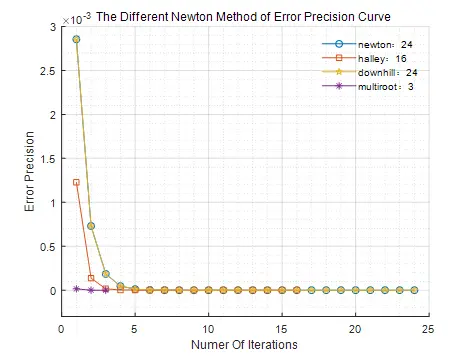
图3 带有重根的牛顿法各迭代方法的精度误差曲线

各方法迭代过程

普通牛顿迭代法
    IterNums     ApproximateSol         ErrorPrecision
    ________    _________________    ____________________
        1       0.947892373805653     0.00285545902358852
        2       0.973327008365232    0.000730340585354261
        3       0.986493966243405    0.000184871077568705
        4       0.993202483991711    4.65199555944595e-05
        5       0.996589832769599    1.16688756544026e-05
        6       0.998292027147433    2.92215229613646e-06
        7       0.999145286557988    7.31159377154178e-07
        8          0.999572460931    1.82867799680686e-07
        9       0.999786184803889    4.57267127496053e-08
       10       0.999893080977268    1.14328996270174e-08
       11       0.999946537631102    2.85837764568697e-09
       12        0.99997326810061    7.14613479502191e-10
       13       0.999986633870396    1.78655867877353e-10
       14       0.999993316892757    4.46641612583676e-11
       15        0.99999665843075      1.116617909247e-11
       16       0.999998329221071    2.79143375081503e-12
       17       0.999999164587949    6.97886193279373e-13
       18       0.999999582277231    1.74527059471075e-13
       19       0.999999791180077    4.36317648677687e-14
       20       0.999999895652271    1.08801856413265e-14
       21       0.999999947786534    2.66453525910038e-15
       22       0.999999973302319     7.7715611723761e-16
       23       0.999999987857067    1.11022302462516e-16
       24       0.999999992428546                       0
牛顿—哈利迭代法
    IterNums     ApproximateSol         ErrorPrecision
    ________    _________________    ____________________
        1       0.965551810226976     0.00122732199318976
        2       0.988384456906306    0.000136484986290042
        3       0.996113110670598    1.51665933865175e-05
        4       0.998702689489662    1.68519748056095e-06
        5       0.999567376081915    1.87244420080113e-07
        6       0.999855771228448    2.08049387717679e-08
        7       0.999951921431764    2.31165986352977e-09
        8       0.999983973553835    2.56851095947752e-10
        9       0.999994657822902    2.85390600041069e-11
       10       0.999998219279682    3.17101900293437e-12
       11       0.999999406450421    3.52273765713562e-13
       12        0.99999980210885     3.9190872769268e-14
       13       0.999999934170877    4.32986979603811e-15
       14       0.999999978008308    4.44089209850063e-16
       15       0.999999991113451    1.11022302462516e-16
       16        1.00000000074541                       0
简化的牛顿迭代法
    IterNums     ApproximateSol         ErrorPrecision
    ________    _________________    ____________________
        1       0.947892373805653     0.00285545902358852
        2       0.960343476131293     0.00163459314954228
        3       0.967471047004351     0.00109236613692898
        4       0.972234261057016    0.000792242820659372
        5       0.975688800710815    0.000605344947669506
        6       0.978328380485372    0.000479800603124803
        7       0.980420529718144    0.000390837064078497
        8       0.982124757387774    0.000325218857110121
        9       0.983542859778547    0.000275282449072156
       10       0.984743216678623    0.000236311720020921
       ......
      196       0.998877331341468    1.26179964665685e-06
      197       0.998882833362819    1.24945532808951e-06
      198       0.998888281557317     1.2372916339265e-06
      199       0.998893676712566    1.22530505242135e-06
      200       0.998899019600859    1.21349215642663e-06
牛顿下山迭代法
    IterNums     ApproximateSol         ErrorPrecision
    ________    _________________    ____________________
        1       0.947892373805653     0.00285545902358852
        2       0.973327008365232    0.000730340585354261
        3       0.986493966243405    0.000184871077568705
        4       0.993202483991711    4.65199555944595e-05
        5       0.996589832769599    1.16688756544026e-05
        6       0.998292027147433    2.92215229613646e-06
        7       0.999145286557988    7.31159377154178e-07
        8          0.999572460931    1.82867799680686e-07
        9       0.999786184803889    4.57267127496053e-08
       10       0.999893080977268    1.14328996270174e-08
       11       0.999946537631102    2.85837764568697e-09
       12        0.99997326810061    7.14613479502191e-10
       13       0.999986633870396    1.78655867877353e-10
       14       0.999993316892757    4.46641612583676e-11
       15        0.99999665843075      1.116617909247e-11
       16       0.999998329221071    2.79143375081503e-12
       17       0.999999164587949    6.97886193279373e-13
       18       0.999999582277231    1.74527059471075e-13
       19       0.999999791180077    4.36317648677687e-14
       20       0.999999895652271    1.08801856413265e-14
       21       0.999999947786534    2.66453525910038e-15
       22       0.999999973302319     7.7715611723761e-16
       23       0.999999987857067    1.11022302462516e-16
       24       0.999999992428546                       0
牛顿重根情形迭代法
    IterNums     ApproximateSol         ErrorPrecision
    ________    _________________    ____________________
       1         1.00384144150858    1.46999496749567e-05
       2         1.00000745433781     5.5566884427094e-11
       3        0.999999999988474                       0

例3：求非线性方程在 $x_0=1$ 附近的近似解：

$f(x)=2e^{-x}sinx=0$

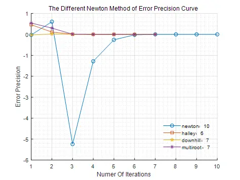
图4 各牛顿迭代法求解非线性方程误差精度下降曲线

其中下山法由于在第二次迭代时引入了下山因子0.25，故其下降曲线相对于牛顿法而言，保持了下降收敛的性质。

&gt;&gt; sol_downhill
sol_downhill =
  包含以下字段的 struct:

           ApproximateSolution: 3.141592653589793
                ErrorPrecision: 1.058435733606881e-17
             NumerOfIterations: 7
                  NewtonMethod: &quot;downhill&quot;
    IntrationProcessInfomation: [7×3 double]
                   convergence: &quot;收敛到满足精度的近似解&quot;
                DownhillLambda: [1 0.250000000000000 1 1 1 1 1]

返回上级列表

请

联系我们

，获取更多内容

< 上一篇: 数学建模技巧：蒙特卡罗法详解及MATLAB代码‌

下一篇: MATLAB串口通信：获取串口端口的函数接口‌ >