该激波/边界层干扰算例是由DLR的Schulein等人设计的。 (Schulein, E., Krogmann, P., and Stanewsky, E., "Documentation of Two-Dimensional Impinging Shock/Turbulent Boundary Layer Interaction Flow", DLR Report DLR IB 223-96 A 49, October 1996.)来流马赫数为5.0,激波由一块10度尖劈产生,并撞击到长500毫米长的平板上,与平板上的湍流边界层发生相互干扰。计算得到的摩擦力曲线将与实验数据进行比较。
表 1 Ma5激波/边界层干扰计算参数
| 参数 | 参数值 |
| 马赫数 | 5.0 |
| 尖劈角度 | 10° |
| 来流静温 | 68.3 K |
| 来流静压 | 4.01×10³ Pa |

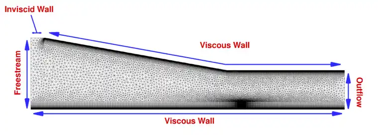
图1 计算网格
计算网格([http://www.grc.nasa.gov/WWW/wind/valid/m5swbli/study01/]{.underline}m5swbli1.tar)为非结构网格,包括近壁区的四边形网格和空间的三角形网格。四边形网格约4.1万,四边形网格约1.9万。激波/边界层干扰区流场梯度大,对该区域网格沿流向适当加密。
下面以SA模型为例,介绍Ma5激波/边界层干扰算例的参数设置。
+-----------------------------------------------------------------------+
| \% ------------- DIRECT, ADJOINT, AND LINEARIZED PROBLEM |
| DEFINITION ------------% |
| |
| \% |
| |
| \% Physical governing equations (EULER, NAVIER_STOKES, |
| |
| \% WAVE_EQUATION, HEAT_EQUATION, FEM_ELASTICITY, |
| |
| \% POISSON_EQUATION) |
| |
| PHYSICAL_PROBLEM= NAVIER_STOKES |
| |
| \% |
| |
| \% Specify turbulent model (NONE, SA, SA_NEG, SST) |
| |
| KIND_TURB_MODEL= SA |
| |
| \% |
| |
| \% Mathematical problem (DIRECT, CONTINUOUS_ADJOINT) |
| |
| MATH_PROBLEM= DIRECT |
| |
| \% |
| |
| \% Restart solution (NO, YES) |
| |
| RESTART_SOL= NO |
| |
| \% -------------------- COMPRESSIBLE FREE-STREAM |
| DEFINITION --------------------% |
| |
| \% |
| |
| \% Mach number (non-dimensional, based on the free-stream values) |
| |
| MACH_NUMBER= 5.0 |
| |
| \% |
| |
| \% Angle of attack (degrees, only for compressible flows) |
| |
| AOA= 0.0 |
| |
| \% |
| |
| \% Free-stream pressure (101325.0 N/m\^2 by default, only Euler |
| flows) |
| |
| FREESTREAM_PRESSURE= 4.01E+03 |
| |
| \% |
| |
| \% Free-stream temperature (273.15 K by default) |
| |
| FREESTREAM_TEMPERATURE= 6.83E+01 |
| |
| \% |
| |
| \% Free-stream temperature (1.2886 Kg/m3 by default) |
| |
| FREESTREAM_DENSITY= 2.04E-01 |
| |
| \% |
| |
| \% Free-stream option to choose if you want to use Density |
| (DENSITY_FS) or Temperature (TEMPERATURE_FS) to initialize the |
| solution |
| |
| FREESTREAM_OPTION= TEMPERATURE_FS |
| |
| \% |
| |
| \%Init option to choose between Reynolds (default) or thermodynamics |
| quantities for initializing the solution (REYNOLDS, TD_CONDITIONS) |
| |
| INIT_OPTION= TD_CONDITIONS |
| |
| \% |
| |
| \% Compressible flow non-dimensionalization (DIMENSIONAL, |
| FREESTREAM_PRESS_EQ_ONE, |
| |
| \% FREESTREAM_VEL_EQ_MACH, FREESTREAM_VEL_EQ_ONE) |
| |
| REF_DIMENSIONALIZATION= FREESTREAM_PRESS_EQ_ONE |
| |
| \% ---------------------- REFERENCE VALUE |
| DEFINITION ---------------------------% |
| |
| \% |
| |
| \% Reference origin for moment computation |
| |
| REF_ORIGIN_MOMENT_X = 0.00 |
| |
| REF_ORIGIN_MOMENT_Y = 0.00 |
| |
| REF_ORIGIN_MOMENT_Z = 0.00 |
| |
| \% |
| |
| \% Reference length for pitching, rolling, and yawing non-dimensional |
| moment |
| |
| REF_LENGTH= 1.0 |
| |
| \% |
| |
| \% Reference area for force coefficients (0 implies automatic |
| calculation) |
| |
| REF_AREA= 1.0 |
| |
| \% -------------------- BOUNDARY CONDITION |
| DEFINITION --------------------------% |
| |
| \% |
| |
| \% Navier-Stokes wall boundary marker(s) (NONE = no marker) |
| |
| \%MARKER_HEATFLUX= ( wall, 0.0 ) |
| |
| \% Format: ( marker name, constant wall temperature (K), ... ) |
| |
| MARKER_ISOTHERMAL= ( wall-up,300,wall-down,300 ) |
| |
| \% Format: (inlet marker, temperature, static pressure, velocity_x, |
| |
| \% velocity_y, velocity_z, ... ), i.e. primitive variables |
| specified. |
| |
| MARKER_SUPERSONIC_INLET= ( inlet, 6.83E+01,4.01E+03,8.28E+02,0,0 ) |
| |
| MARKER_SUPERSONIC_OUTLET= ( outlet ) |
| |
| MARKER_SYM= ( Symmetry ) |
| |
| \% |
| |
| \% Farfield boundary marker(s) (NONE = no marker) |
| |
| \%MARKER_FAR= ( FARFIELD ) |
| |
| \% |
| |
| \% Marker(s) of the surface to be plotted or designed |
| |
| MARKER_PLOTTING= ( wall-down ) |
| |
| \% |
| |
| \% Marker(s) of the surface where the functional (Cd, Cl, etc.) will |
| be evaluated |
| |
| MARKER_MONITORING= ( wall-up,wall-down ) |
| |
| \% ------------- COMMON PARAMETERS DEFINING THE NUMERICAL |
| METHOD ---------------% |
| |
| \% |
| |
| \% Numerical method for spatial gradients (GREEN_GAUSS, |
| WEIGHTED_LEAST_SQUARES) |
| |
| NUM_METHOD_GRAD= GREEN_GAUSS |
| |
| \% |
| |
| \% Courant-Friedrichs-Lewy condition of the finest grid |
| |
| CFL_NUMBER= 10 |
| |
| \% |
| |
| \% Adaptive CFL number (NO, YES) |
| |
| CFL_ADAPT= YES |
| |
| \% |
| |
| \% Parameters of the adaptive CFL number (factor down, factor up, CFL |
| min value, |
| |
| \% CFL max value ) |
| |
| CFL_ADAPT_PARAM= ( 1.5, 0.5, 1.0, 100.0 ) |
| |
| \% |
| |
| \% Number of total iterations |
| |
| EXT_ITER= 10000 |
| |
| \% |
| |
| \% Linear solver for the implicit formulation (BCGSTAB, FGMRES) |
| |
| LINEAR_SOLVER= BCGSTAB |
| |
| \% |
| |
| \% Min error of the linear solver for the implicit formulation |
| |
| LINEAR_SOLVER_ERROR= 1E-6 |
| |
| \% |
| |
| \% Max number of iterations of the linear solver for the implicit |
| formulation |
| |
| LINEAR_SOLVER_ITER= 20 |
| |
| \% -------------------------- MULTIGRID |
| PARAMETERS -----------------------------% |
| |
| \% |
| |
| \% Multi-Grid Levels (0 = no multi-grid) |
| |
| MGLEVEL= 0 |
| |
| \% |
| |
| \% Multi-grid cycle (V_CYCLE, W_CYCLE, FULLMG_CYCLE) |
| |
| MGCYCLE= W_CYCLE |
| |
| \% |
| |
| \% Multi-grid pre-smoothing level |
| |
| MG_PRE_SMOOTH= ( 1, 2, 3, 3 ) |
| |
| \% |
| |
| \% Multi-grid post-smoothing level |
| |
| MG_POST_SMOOTH= ( 0, 0, 0, 0 ) |
| |
| \% |
| |
| \% Jacobi implicit smoothing of the correction |
| |
| MG_CORRECTION_SMOOTH= ( 0, 0, 0, 0 ) |
| |
| \% |
| |
| \% Damping factor for the residual restriction |
| |
| MG_DAMP_RESTRICTION= 0.95 |
| |
| \% |
| |
| \% Damping factor for the correction prolongation |
| |
| MG_DAMP_PROLONGATION= 0.95 |
| |
| \% -------------------- FLOW NUMERICAL METHOD |
| DEFINITION -----------------------% |
| |
| \% |
| |
| \% Convective numerical method (JST, LAX-FRIEDRICH, CUSP, ROE, AUSM, |
| HLLC, |
| |
| \% TURKEL_PREC, MSW) |
| |
| CONV_NUM_METHOD_FLOW= JST |
| |
| \% |
| |
| \% Monotonic Upwind Scheme for Conservation Laws (TVD) in the flow |
| equations. |
| |
| \% Required for 2nd order upwind schemes (NO, YES) |
| |
| MUSCL_FLOW= YES |
| |
| \% |
| |
| \% Slope limiter (VENKATAKRISHNAN, MINMOD) |
| |
| SLOPE_LIMITER_FLOW= VENKATAKRISHNAN |
| |
| \% |
| |
| \% Coefficient for the limiter (smooth regions) |
| |
| VENKAT_LIMITER_COEFF= 0.03 |
| |
| \% |
| |
| \% 2nd and 4th order artificial dissipation coefficients |
| |
| JST_SENSOR_COEFF= ( 0.5, 0.02 ) |
| |
| \% |
| |
| \% Time discretization (RUNGE-KUTTA_EXPLICIT, EULER_IMPLICIT, |
| EULER_EXPLICIT) |
| |
| TIME_DISCRE_FLOW= EULER_IMPLICIT |
| |
| \% -------------------- TURBULENT NUMERICAL METHOD |
| DEFINITION ------------------% |
| |
| \% |
| |
| \% Convective numerical method (SCALAR_UPWIND) |
| |
| CONV_NUM_METHOD_TURB= SCALAR_UPWIND |
| |
| \% |
| |
| \% Monotonic Upwind Scheme for Conservation Laws (TVD) in the |
| turbulence equations. |
| |
| \% Required for 2nd order upwind schemes (NO, YES) |
| |
| MUSCL_TURB= NO |
| |
| \% |
| |
| \% Time discretization (EULER_IMPLICIT) |
| |
| TIME_DISCRE_TURB= EULER_IMPLICIT |
| |
| \% ---------------- ADJOINT-FLOW NUMERICAL METHOD |
| DEFINITION -------------------% |
| |
| \% Adjoint problem boundary condition (DRAG, LIFT, SIDEFORCE, |
| MOMENT_X, |
| |
| \% MOMENT_Y, MOMENT_Z, EFFICIENCY, |
| |
| \% EQUIVALENT_AREA, NEARFIELD_PRESSURE, |
| |
| \% FORCE_X, FORCE_Y, FORCE_Z, THRUST, |
| |
| \% TORQUE, FREE_SURFACE, TOTAL_HEAT, |
| |
| \% MAXIMUM_HEATFLUX, INVERSE_DESIGN_PRESSURE, |
| |
| \% INVERSE_DESIGN_HEATFLUX) |
| |
| OBJECTIVE_FUNCTION= DRAG |
| |
| \% |
| |
| \% Convective numerical method (JST, LAX-FRIEDRICH, ROE) |
| |
| CONV_NUM_METHOD_ADJFLOW= JST |
| |
| \% |
| |
| \% Monotonic Upwind Scheme for Conservation Laws (TVD) in the adjoint |
| flow equations. |
| |
| \% Required for 2nd order upwind schemes (NO, YES) |
| |
| MUSCL_ADJFLOW= YES |
| |
| \% |
| |
| \% Slope limiter (NONE, VENKATAKRISHNAN, BARTH_JESPERSEN, |
| VAN_ALBADA_EDGE, |
| |
| \% SHARP_EDGES, WALL_DISTANCE) |
| |
| SLOPE_LIMITER_ADJFLOW= NONE |
| |
| \% |
| |
| \% Coefficient for the sharp edges limiter |
| |
| ADJ_SHARP_LIMITER_COEFF= 3.0 |
| |
| \% |
| |
| \% 2nd, and 4th order artificial dissipation coefficients |
| |
| ADJ_JST_SENSOR_COEFF= ( 0.0, 0.01 ) |
| |
| \% |
| |
| \% Reduction factor of the CFL coefficient in the adjoint problem |
| |
| CFL_REDUCTION_ADJFLOW= 0.75 |
| |
| \% |
| |
| \% Time discretization (RUNGE-KUTTA_EXPLICIT, EULER_IMPLICIT) |
| |
| TIME_DISCRE_ADJFLOW= EULER_IMPLICIT |
| |
| \% |
| |
| \% Adjoint frozen viscosity (NO, YES) |
| |
| FROZEN_VISC_CONT= YES |
| |
| \% --------------------------- CONVERGENCE |
| PARAMETERS --------------------------% |
| |
| \% |
| |
| \% Convergence criteria (CAUCHY, RESIDUAL) |
| |
| \% |
| |
| CONV_CRITERIA= RESIDUAL |
| |
| \% |
| |
| \% Residual reduction (order of magnitude with respect to the initial |
| value) |
| |
| RESIDUAL_REDUCTION= 8 |
| |
| \% |
| |
| \% Min value of the residual (log10 of the residual) |
| |
| RESIDUAL_MINVAL= -8 |
| |
| \% |
| |
| \% Start convergence criteria at iteration number |
| |
| STARTCONV_ITER= 10 |
| |
| \% |
| |
| \% Number of elements to apply the criteria |
| |
| CAUCHY_ELEMS= 100 |
| |
| \% |
| |
| \% Epsilon to control the series convergence |
| |
| CAUCHY_EPS= 1E-6 |
| |
| \% |
| |
| \% Function to apply the criteria (LIFT, DRAG, NEARFIELD_PRESS, |
| SENS_GEOMETRY, |
| |
| \% SENS_MACH, DELTA_LIFT, DELTA_DRAG) |
| |
| CAUCHY_FUNC_FLOW= DRAG |
| |
| \% ------------------------- INPUT/OUTPUT |
| INFORMATION --------------------------% |
| |
| \% |
| |
| \% Mesh input file |
| |
| MESH_FILENAME= swbli.su2 |
| |
| \% |
| |
| \% Mesh input file format (SU2, CGNS, NETCDF_ASCII) |
| |
| MESH_FORMAT= SU2 |
| |
| \% |
| |
| \% Mesh output file |
| |
| MESH_OUT_FILENAME= mesh_out.su2 |
| |
| \% |
| |
| \% Restart flow input file |
| |
| SOLUTION_FLOW_FILENAME= restart_flow.dat |
| |
| \% |
| |
| \% Restart adjoint input file |
| |
| SOLUTION_ADJ_FILENAME= solution_adj.dat |
| |
| \% |
| |
| \% Output file format (PARAVIEW, TECPLOT, STL) |
| |
| OUTPUT_FORMAT= TECPLOT |
| |
| \% |
| |
| \% Output file convergence history (w/o extension) |
| |
| CONV_FILENAME= history |
| |
| \% |
| |
| \% Output file restart flow |
| |
| RESTART_FLOW_FILENAME= restart_flow.dat |
| |
| \% |
| |
| \% Output file restart adjoint |
| |
| RESTART_ADJ_FILENAME= restart_adj.dat |
| |
| \% |
| |
| \% Output file flow (w/o extension) variables |
| |
| VOLUME_FLOW_FILENAME= flow |
| |
| \% |
| |
| \% Output file adjoint (w/o extension) variables |
| |
| VOLUME_ADJ_FILENAME= adjoint |
| |
| \% |
| |
| \% Output objective function gradient (using continuous adjoint) |
| |
| GRAD_OBJFUNC_FILENAME= of_grad.dat |
| |
| \% |
| |
| \% Output file surface flow coefficient (w/o extension) |
| |
| SURFACE_FLOW_FILENAME= surface_flow |
| |
| \% |
| |
| \% Output file surface adjoint coefficient (w/o extension) |
| |
| SURFACE_ADJ_FILENAME= surface_adjoint |
| |
| \% |
| |
| \% Writing solution file frequency |
| |
| WRT_SOL_FREQ= 2000 |
| |
| \% |
| |
| \% Writing convergence history frequency |
| |
| WRT_CON_FREQ= 1 |
+-----------------------------------------------------------------------+
图2展示了SU2计算的Ma5激波/边界层干扰流场。可以看到,尖劈头部形成的激波撞击到下侧的平板边界层后向上反射,并与膨胀波相互作用。

图 2 激波/边界层干扰流场马赫数云图

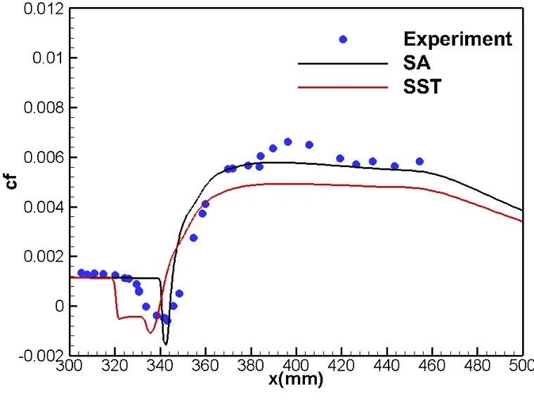
图 3 激波/边界层干扰区摩檫力系数分布

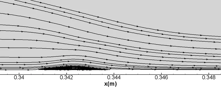
(a)SA模型

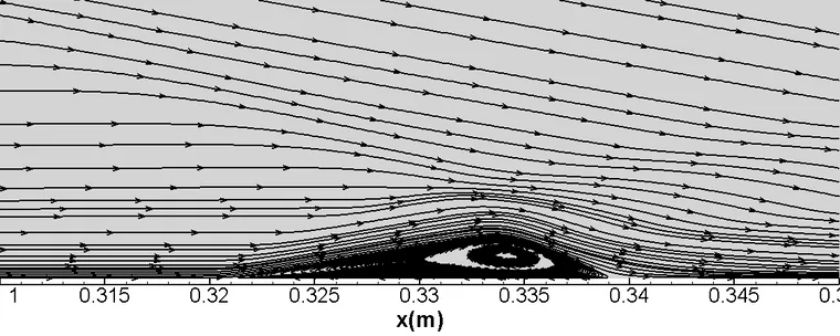
(b)SST模型
图 4 激波/边界层干扰区流线
图3展示了两种湍流模型计算的摩擦力曲线与试验的对比结果。计算得到的摩檫力系数与试验结果相比,量级相当,趋势也基本保持一致。此外,从图4可以看出,SA模型计算得到的分离区范围跟SST相比明显偏小。
采用SU2计算了Ma5激波/边界层干扰流场。计算得到的摩檫力系数与试验结果相比,量级相当,趋势也基本保持一致。SA模型计算得到的分离区范围跟SST相比明显偏小。
免责声明:本文系网络转载或改编,未找到原创作者,版权归原作者所有。如涉及版权,请联系删
武汉格发信息技术有限公司,格发许可优化管理系统可以帮你评估贵公司软件许可的真实需求,再低成本合规性管理软件许可,帮助贵司提高软件投资回报率,为软件采购、使用提供科学决策依据。支持的软件有: CAD,CAE,PDM,PLM,Catia,Ugnx, AutoCAD, Pro/E, Solidworks ,Hyperworks, Protel,CAXA,OpenWorks LandMark,MATLAB,Enovia,Winchill,TeamCenter,MathCAD,Ansys, Abaqus,ls-dyna, Fluent, MSC,Bentley,License,UG,ug,catia,Dassault Systèmes,AutoDesk,Altair,autocad,PTC,SolidWorks,Ansys,Siemens PLM Software,Paradigm,Mathworks,Borland,AVEVA,ESRI,hP,Solibri,Progman,Leica,Cadence,IBM,SIMULIA,Citrix,Sybase,Schlumberger,MSC Products...