TensorFlow深度学习：逆归一化与回归预测

实验目的

1.掌握使用TensorFlow进行逻辑回归

2.掌握逻辑回归的原理

实验原理

逻辑回归是机器学习中很简答的一个例子，这篇文章就是要介绍如何使用tensorflow实现一个简单的逻辑回归算法。

逻辑回归可以看作只有一层网络的前向神经网络，并且参数连接的权重只是一个值，而非矩阵。公式为：y_predict=logistic(X*W+b)，其中X为输入，W为输入与隐含层之间的权重，b为隐含层神经元的偏置，而logistic为激活函数，一般为sigmoid或者tanh，y_predict为最终预测结果。

逻辑回归是一种分类器模型，需要函数不断的优化参数，这里目标函数为y_predict与真实标签Y之间的L2距离，使用随机梯度下降算法来更新权重和偏置。

实验步骤

1、导入实验所需要的模块

import tensorflow as tf
from tensorflow.examples.tutorials.mnist import input_data

2、导入实验所需的数据

mnist = input_data.read_data_sets("D:/jqxx/mnist/",one_hot = True)

3、设置训练参数

learning_rate=0.01
training_epochs=25
batch_size=100
display_step=1

4、构造计算图，使用占位符placeholder函数构造变量x，y，代码如下：

x=tf.placeholder(tf.float32,[None,784])
y=tf.placeholder(tf.float32,[None,10])

5、使用Variable函数，设置模型的初始权重

W=tf.Variable(tf.zeros([784,10]))
b=tf.Variable(tf.zeros([10]))

6、构造逻辑回归模型

pred=tf.nn.softmax(tf.matmul(x,W)+b)

7、构造代价函数cost

cost=tf.reduce_mean(-tf.reduce_sum(y*tf.log(pred),reduction_indices=1))

8、使用梯度下降法求最小值，即最优解

optimizer=tf.train.GradientDescentOptimizer(learning_rate).minimize(cost)

9、初始化全部变量

init=tf.global_variables_initializer()

10、使用tf.Session()创建Session会话对象，会话封装了Tensorflow运行时的状态和控制。

with tf.Session() as sess:
    sess.run(init)
    

11、调用会话对象sess的run方法，运行计算图，即开始训练模型。

for epoch in range(training_epochs):
        avg_cost = 0
        total_batch = int(mnist.train.num_examples / batch_size)
        for i in range(total_batch):
            batch_xs, batch_ys = mnist.train.next_batch(batch_size)
            _, c = sess.run([optimizer, cost], feed_dict={x: batch_xs, y: batch_ys})
            avg_cost += c  / total_batch
        if (epoch+1) % display_step == 0:
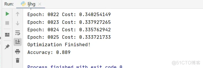
            print("Epoch:", '%04d' % (epoch + 1), "Cost:","{:.09f}".format(avg_cost))
    print("Optimization Finished!")
    

12、测试模型

correct_prediction = tf.equal(tf.argmax(pred, 1), tf.argmax(y, 1))

13、评估模型的准确度。

accuracy = tf.reduce_mean(tf.cast(correct_prediction, tf.float32))
    print("Accuracy:", accuracy.eval（{x: mnist.test.images[:3000], 
    y: mnist.test.labels[:3000]}))
    

14、完整代码：

import tensorflow as tf
from tensorflow.examples.tutorials.mnist import input_data

#导入实验所需的数据

mnist = input_data.read_data_sets("D:/jqxx/mnist/",one_hot = True)

#设置训练参数
learning_rate=0.01
training_epochs=25
batch_size=100
display_step=1

#构造计算图，使用占位符placeholder函数构造变量x，y，
x=tf.placeholder(tf.float32,[None,784])
y=tf.placeholder(tf.float32,[None,10])

# 使用Variable函数，设置模型的初始权重
W=tf.Variable(tf.zeros([784,10]))
b=tf.Variable(tf.zeros([10]))
#构造逻辑回归模型
pred=tf.nn.softmax(tf.matmul(x,W)+b)
#构造代价函数cost
cost=tf.reduce_mean(-tf.reduce_sum(y*tf.log(pred),reduction_indices=1))
#使用梯度下降法求最小值，即最优解
optimizer=tf.train.GradientDescentOptimizer(learning_rate).minimize(cost)
#初始化全部变量
init=tf.global_variables_initializer()
#.使用tf.Session()创建Session会话对象，会话封装了Tensorflow运行时的状态和控制
with tf.Session() as sess:
    sess.run(init)
    #调用会话对象sess的run方法，运行计算图，即开始训练模型
    for epoch in range(training_epochs):
        avg_cost = 0
        total_batch = int(mnist.train.num_examples / batch_size)
        for i in range(total_batch):
            batch_xs, batch_ys = mnist.train.next_batch(batch_size)
            _, c = sess.run([optimizer, cost], feed_dict={x: batch_xs, y: batch_ys})
            avg_cost += c  / total_batch
        if (epoch+1) % display_step == 0:
            print("Epoch:", '%04d' % (epoch + 1), "Cost:","{:.09f}".format(avg_cost))
    print("Optimization Finished!")
    #测试模型
    correct_prediction = tf.equal(tf.argmax(pred, 1), tf.argmax(y, 1))
    #评估模型的准确度
    accuracy = tf.reduce_mean(tf.cast(correct_prediction, tf.float32))
    print("Accuracy:", accuracy.eval（{x: mnist.test.images[:3000], y: 
    mnist.test.labels[:3000]}))
    

View Code

15、运行结果为：

免责声明：本文系网络转载或改编，未找到原创作者，版权归原作者所有。如涉及版权，请联系删