二维超声速空腔
空腔外形在内埋武器舱、起落架舱、超燃冲压发动机燃烧室等先进飞行器部件中有着广泛应用。本文以参考文献(Zhang and Rona, 1998, Journal of Sound and Vibration)提供的空腔外形为对象,采用ddes方法计算二维超声速空腔流动,检验SU2对于超声速非定常流场的模拟能力。
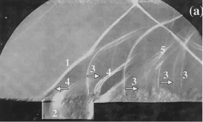
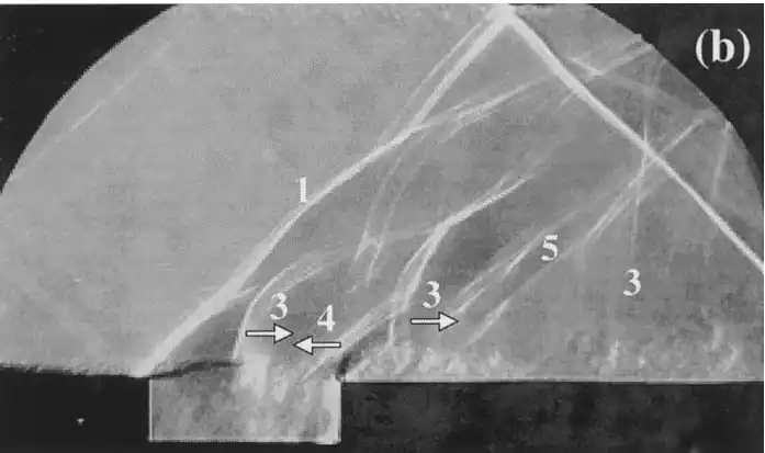
图 1 二维超声速空腔试验纹影结果
表 1 二维超声速空腔试验参数
| 参数名称 | 参数值 |
| 马赫数 | 1.5 |
| 空腔长度L | 0.045 m |
| 空腔深度D | 0.015 m |
| 空腔宽度W | 0.114 m |
| 雷诺数Re(参考长度为L) |
计算网格直接在pointwise软件中生成,网格包括空腔内部及平板上方两个网格块。空腔内部网格块为321×149个网格点,平板上方网格块为1011×359个网格点。平板上方边界层内第一层网格高度为4.5×10^-7^米。

a)二维空腔流动全局计算网格(i,j方向每8个网格点显示1个)
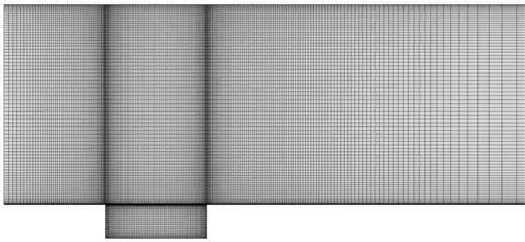
(b)二维空腔流动局部计算网格(i,j方向每4个网格点显示1个)
图 2 二维超声速空腔试验纹影结果
下面介绍二维超声速空腔算例的参数设置。
+-----------------------------------------------------------------------+
| \% ------------- DIRECT, ADJOINT, AND LINEARIZED PROBLEM |
| DEFINITION ------------% |
| |
| \% |
| |
| \% Physical governing equations (EULER, NAVIER_STOKES, |
| |
| \% WAVE_EQUATION, HEAT_EQUATION, FEM_ELASTICITY, |
| |
| \% POISSON_EQUATION) |
| |
| PHYSICAL_PROBLEM= NAVIER_STOKES |
| |
| \% |
| |
| \% Specify turbulent model (NONE, SA, SA_NEG, SST) |
| |
| KIND_TURB_MODEL= SA |
| |
| HYBRID_RANSLES= SA_EDDES |
| |
| \% |
| |
| \% Mathematical problem (DIRECT, CONTINUOUS_ADJOINT) |
| |
| MATH_PROBLEM= DIRECT |
| |
| \% |
| |
| \% Restart solution (NO, YES) |
| |
| RESTART_SOL= NO |
| |
| \%initialization |
| |
| TESTCASE_TYPE= CAVITY |
| |
| \% -------------------- COMPRESSIBLE FREE-STREAM |
| DEFINITION --------------------% |
| |
| \% |
| |
| \% Mach number (non-dimensional, based on the free-stream values) |
| |
| MACH_NUMBER= 1.5 |
| |
| \% |
| |
| \% Angle of attack (degrees, only for compressible flows) |
| |
| AOA= 0.0 |
| |
| \% |
| |
| \% Init option to choose between Reynolds (default) or thermodynamics |
| quantities |
| |
| \% for initializing the solution (REYNOLDS, TD_CONDITIONS) |
| |
| INIT_OPTION= REYNOLDS |
| |
| \% |
| |
| \% Free-stream option to choose between density and temperature |
| (default) for |
| |
| \% initializing the solution (TEMPERATURE_FS, DENSITY_FS) |
| |
| FREESTREAM_OPTION= TEMPERATURE_FS |
| |
| \% |
| |
| \% Free-stream pressure (101325.0 N/m\^2, 2116.216 psf by default) |
| |
| FREESTREAM_PRESSURE= 5.38E4 |
| |
| \% |
| |
| \% Free-stream temperature (288.15 K by default) |
| |
| FREESTREAM_TEMPERATURE= 200 |
| |
| \% |
| |
| \% Reynolds number (non-dimensional, based on the free-stream values) |
| |
| REYNOLDS_NUMBER= 1.35E6 |
| |
| \% |
| |
| \% Reynolds length (1 m by default) |
| |
| REYNOLDS_LENGTH= 0.045 |
| |
| \% |
|
| \% Compressible flow non-dimensionalization (DIMENSIONAL, |
| FREESTREAM_PRESS_EQ_ONE,
| |
| \% FREESTREAM_VEL_EQ_MACH, FREESTREAM_VEL_EQ_ONE) |
| |
| REF_DIMENSIONALIZATION= FREESTREAM_VEL_EQ_ONE |
| |
| \% ---------------------- REFERENCE VALUE |
| DEFINITION ---------------------------% |
| |
| \% |
| |
| \% Reference origin for moment computation |
| |
| REF_ORIGIN_MOMENT_X = 0.25 |
| |
| REF_ORIGIN_MOMENT_Y = 0.00 |
| |
| REF_ORIGIN_MOMENT_Z = 0.00 |
| |
| \% |
| |
| \% Reference length for pitching, rolling, and yawing non-dimensional |
| moment |
| |
| REF_LENGTH= 1.0 |
| |
| \% |
| |
| \% Reference area for force coefficients (0 implies automatic |
| calculation) |
| |
| REF_AREA= 0.045 |
| |
| \% ------------------------- UNSTEADY |
| SIMULATION |
| -------------------------------% |
| |
| \% |
| |
| \% Unsteady simulation (NO, TIME_STEPPING, |
| DUAL_TIME_STEPPING-1ST_ORDER, |
| |
| \% DUAL_TIME_STEPPING-2ND_ORDER, TIME_SPECTRAL) |
| |
| \%UNSTEADY_SIMULATION= NO |
| |
| UNSTEADY_SIMULATION= DUAL_TIME_STEPPING-2ND_ORDER |
| |
| \% |
| |
| \% Time Step for dual time stepping simulations (s) |
| |
| \% U_inf = 425 - L=4.5E-2 dt=0.002 - |
| |
| UNST_TIMESTEP= 2.12E-7 |
| |
| \% |
| |
| \% Total Physical Time for dual time stepping simulations (s) |
| |
| UNST_TIME= 1.06E-2 |
| |
| \% |
| |
| \% Unsteady Courant-Friedrichs-Lewy number of the finest grid |
| |
| UNST_CFL_NUMBER= 0.0 |
| |
| \% |
| |
| \% Number of internal iterations (dual time method) |
| |
| UNST_INT_ITER= 30 |
| |
| \% |
| |
| \% Iteration number to begin unsteady restarts |
| |
| UNST_RESTART_ITER= 2 |
| |
| \% -------------------- BOUNDARY CONDITION |
| DEFINITION --------------------------% |
| |
| \% |
| |
| \% Navier-Stokes wall boundary marker(s) (NONE = no marker) |
| |
| MARKER_HEATFLUX= ( wall-down, 0.0 ) |
| |
| \% Format: (inlet marker, temperature, static pressure, velocity_x, |
| |
| \% velocity_y, velocity_z, ... ), i.e. primitive variables |
| specified. |
| |
| MARKER_SUPERSONIC_INLET= ( inlet, 200,5.38E4,425.22,0,0 ) |
| |
| MARKER_SUPERSONIC_OUTLET= ( outlet ) |
| |
| MARKER_SYM= ( wall-up ) |
| |
| \% |
| |
| \% Farfield boundary marker(s) (NONE = no marker) |
| |
| \%MARKER_FAR= ( FARFIELD ) |
| |
| \% |
| |
| \% Marker(s) of the surface to be plotted or designed |
| |
| MARKER_PLOTTING= ( wall-down ) |
| |
| \% |
| |
| \% Marker(s) of the surface where the functional (Cd, Cl, etc.) will |
| be evaluated |
| |
| MARKER_MONITORING= ( wall-down ) |
| |
| \% ------------- COMMON PARAMETERS DEFINING THE NUMERICAL |
| METHOD ---------------% |
| |
| \% |
| |
| \% Numerical method for spatial gradients (GREEN_GAUSS, |
| WEIGHTED_LEAST_SQUARES) |
| |
| NUM_METHOD_GRAD= GREEN_GAUSS |
| |
| \% |
| |
| \% Courant-Friedrichs-Lewy condition of the finest grid |
| |
| CFL_NUMBER= 10 |
| |
| \% |
| |
| \% Adaptive CFL number (NO, YES) |
| |
| CFL_ADAPT= NO |
| |
| \% |
| |
| \% Parameters of the adaptive CFL number (factor down, factor up, CFL |
| min value, |
| |
| \% CFL max value ) |
| |
| CFL_ADAPT_PARAM= ( 1.5, 0.5, 1.0, 100.0 ) |
| |
| \% |
| |
| \% Number of total iterations |
| |
| EXT_ITER= 50000 |
| |
| \% |
| |
| \% Linear solver for the implicit formulation (BCGSTAB, FGMRES) |
| |
| LINEAR_SOLVER= BCGSTAB |
| |
| \% |
| |
| \% Min error of the linear solver for the implicit formulation |
| |
| LINEAR_SOLVER_ERROR= 1E-6 |
| |
| \% |
| |
| \% Max number of iterations of the linear solver for the implicit |
| formulation |
| |
| LINEAR_SOLVER_ITER= 20 |
| |
| \% -------------------------- MULTIGRID |
| PARAMETERS -----------------------------% |
| |
| \% |
| |
| \% Multi-Grid Levels (0 = no multi-grid) |
| |
| MGLEVEL= 0 |
| |
| \% |
| |
| \% Multi-grid cycle (V_CYCLE, W_CYCLE, FULLMG_CYCLE) |
| |
| MGCYCLE= W_CYCLE |
| |
| \% |
| |
| \% Multi-grid pre-smoothing level |
| |
| MG_PRE_SMOOTH= ( 1, 2, 3, 3 ) |
| |
| \% |
| |
| \% Multi-grid post-smoothing level |
| |
| MG_POST_SMOOTH= ( 0, 0, 0, 0 ) |
| |
| \% |
| |
| \% Jacobi implicit smoothing of the correction |
| |
| MG_CORRECTION_SMOOTH= ( 0, 0, 0, 0 ) |
| |
| \% |
| |
| \% Damping factor for the residual restriction |
| |
| MG_DAMP_RESTRICTION= 0.95 |
| |
| \% |
| |
| \% Damping factor for the correction prolongation |
| |
| MG_DAMP_PROLONGATION= 0.95 |
| |
| \% -------------------- FLOW NUMERICAL METHOD |
| DEFINITION -----------------------% |
| |
| \% |
| |
| \% Convective numerical method (JST, LAX-FRIEDRICH, CUSP, ROE, AUSM, |
| HLLC, |
| |
| \% TURKEL_PREC, MSW) |
| |
| CONV_NUM_METHOD_FLOW= JST |
| |
| \% |
| |
| \% Monotonic Upwind Scheme for Conservation Laws (TVD) in the flow |
| equations. |
| |
| \% Required for 2nd order upwind schemes (NO, YES) |
| |
| MUSCL_FLOW= YES |
| |
| \% |
| |
| \% Slope limiter (VENKATAKRISHNAN, MINMOD) |
| |
| SLOPE_LIMITER_FLOW= VENKATAKRISHNAN |
| |
| \% |
| |
| \% Coefficient for the limiter (smooth regions) |
| |
| VENKAT_LIMITER_COEFF= 0.03 |
| |
| \% |
| |
| \% 2nd and 4th order artificial dissipation coefficients |
| |
| JST_SENSOR_COEFF= ( 0.5, 0.02 ) |
| |
| \% |
| |
| \% Time discretization (RUNGE-KUTTA_EXPLICIT, EULER_IMPLICIT, |
| EULER_EXPLICIT) |
| |
| TIME_DISCRE_FLOW= EULER_IMPLICIT |
| |
| \% -------------------- TURBULENT NUMERICAL METHOD |
| DEFINITION ------------------% |
| |
| \% |
| |
| \% Convective numerical method (SCALAR_UPWIND) |
| |
| CONV_NUM_METHOD_TURB= SCALAR_UPWIND |
| |
| \% |
| |
| \% Monotonic Upwind Scheme for Conservation Laws (TVD) in the |
| turbulence equations. |
| |
| \% Required for 2nd order upwind schemes (NO, YES) |
| |
| MUSCL_TURB= NO |
| |
| \% |
| |
| \% Time discretization (EULER_IMPLICIT) |
| |
| TIME_DISCRE_TURB= EULER_IMPLICIT |
| |
| \% ---------------- ADJOINT-FLOW NUMERICAL METHOD |
| DEFINITION -------------------% |
| |
| \% Adjoint problem boundary condition (DRAG, LIFT, SIDEFORCE, |
| MOMENT_X, |
| |
| \% MOMENT_Y, MOMENT_Z, EFFICIENCY, |
| |
| \% EQUIVALENT_AREA, NEARFIELD_PRESSURE, |
| |
| \% FORCE_X, FORCE_Y, FORCE_Z, THRUST, |
| |
| \% TORQUE, FREE_SURFACE, TOTAL_HEAT, |
| |
| \% MAXIMUM_HEATFLUX, INVERSE_DESIGN_PRESSURE, |
| |
| \% INVERSE_DESIGN_HEATFLUX) |
| |
| OBJECTIVE_FUNCTION= DRAG |
| |
| \% |
| |
| \% Convective numerical method (JST, LAX-FRIEDRICH, ROE) |
| |
| CONV_NUM_METHOD_ADJFLOW= JST |
| |
| \% |
| |
| \% Monotonic Upwind Scheme for Conservation Laws (TVD) in the adjoint |
| flow equations. |
| |
| \% Required for 2nd order upwind schemes (NO, YES) |
| |
| MUSCL_ADJFLOW= YES |
| |
| \% |
| |
| \% Slope limiter (NONE, VENKATAKRISHNAN, BARTH_JESPERSEN, |
| VAN_ALBADA_EDGE, |
| |
| \% SHARP_EDGES, WALL_DISTANCE) |
| |
| SLOPE_LIMITER_ADJFLOW= NONE |
| |
| \% |
| |
| \% Coefficient for the sharp edges limiter |
| |
| ADJ_SHARP_LIMITER_COEFF= 3.0 |
| |
| \% |
| |
| \% 2nd, and 4th order artificial dissipation coefficients |
| |
| ADJ_JST_SENSOR_COEFF= ( 0.0, 0.01 ) |
| |
| \% |
| |
| \% Reduction factor of the CFL coefficient in the adjoint problem |
| |
| CFL_REDUCTION_ADJFLOW= 0.75 |
| |
| \% |
| |
| \% Time discretization (RUNGE-KUTTA_EXPLICIT, EULER_IMPLICIT) |
| |
| TIME_DISCRE_ADJFLOW= EULER_IMPLICIT |
| |
| \% |
| |
| \% Adjoint frozen viscosity (NO, YES) |
| |
| FROZEN_VISC_CONT= YES |
| |
| \% --------------------------- CONVERGENCE |
| PARAMETERS --------------------------% |
| |
| \% |
| |
| \% Convergence criteria (CAUCHY, RESIDUAL) |
| |
| \% |
| |
| CONV_CRITERIA= RESIDUAL |
| |
| \% |
| |
| \% Residual reduction (order of magnitude with respect to the initial |
| value) |
| |
| RESIDUAL_REDUCTION= 3 |
| |
| \% |
| |
| \% Min value of the residual (log10 of the residual) |
| |
| RESIDUAL_MINVAL= -15 |
| |
| \% |
| |
| \% Start convergence criteria at iteration number |
| |
| STARTCONV_ITER= 10 |
| |
| \% |
| |
| \% Number of elements to apply the criteria |
| |
| CAUCHY_ELEMS= 100 |
| |
| \% |
| \% Epsilon to control the series convergence |
| |
| CAUCHY_EPS= 1E-6 |
| |
| \% |
| |
| \% Function to apply the criteria (LIFT, DRAG, NEARFIELD_PRESS, |
| SENS_GEOMETRY, |
| |
| \% SENS_MACH, DELTA_LIFT, DELTA_DRAG) |
| |
| CAUCHY_FUNC_FLOW= DRAG |
| |
| \% ------------------------- INPUT/OUTPUT |
| INFORMATION --------------------------% |
| |
| \% |
| |
| \% Mesh input file |
| |
| MESH_FILENAME= cavity-LD3-fine.su2 |
| \% |
| |
| \% Mesh input file format (SU2, CGNS, NETCDF_ASCII) |
| |
| MESH_FORMAT= SU2 |
| |
| \% |
| |
| \% Mesh output file |
| |
| MESH_OUT_FILENAME= mesh_out.su2 |
| |
| \% |
| |
| \% Restart flow input file |
| |
| SOLUTION_FLOW_FILENAME= restart_flow.dat |
| |
| \% |
| |
| \% Restart adjoint input file |
| |
| SOLUTION_ADJ_FILENAME= solution_adj.dat |
| |
| \% |
| |
| \% Output file format (PARAVIEW, TECPLOT, STL) |
| |
| OUTPUT_FORMAT= TECPLOT_BINARY |
| |
| \% |
| |
| \% Output file convergence history (w/o extension) |
| |
| CONV_FILENAME= history |
| |
| \% |
| |
| \% Output file restart flow |
| |
| RESTART_FLOW_FILENAME= restart_flow.dat |
| |
| \% |
| |
| \% Output file restart adjoint |
| |
| RESTART_ADJ_FILENAME= restart_adj.dat |
| |
| \% |
| |
| \% Output file flow (w/o extension) variables |
| |
| VOLUME_FLOW_FILENAME= flow |
| |
| \% |
| |
| \% Output file adjoint (w/o extension) variables |
| |
| VOLUME_ADJ_FILENAME= adjoint |
| |
| \% |
| |
| \% Output objective function gradient (using continuous adjoint) |
| |
| GRAD_OBJFUNC_FILENAME= of_grad.dat |
| |
| \% |
| |
| \% Output file surface flow coefficient (w/o extension) |
| |
| SURFACE_FLOW_FILENAME= surface_flow |
| |
| \% |
| |
| \% Output file surface adjoint coefficient (w/o extension) |
| |
| SURFACE_ADJ_FILENAME= surface_adjoint |
| |
| \% |
| |
| \% Writing solution file frequency |
| |
| WRT_SOL_FREQ= 100 |
| |
| \% |
| |
| \% Writing convergence history frequency |
| |
| WRT_CON_FREQ= 1 |
| |
| \% Writing solution file frequency for physical time steps (dual |
| time) |
| |
| WRT_SOL_FREQ_DUALTIME= 30 |
| |
| WRT_SURF_FREQ_DUALTIME= 1 |
+-----------------------------------------------------------------------+
在算例cfg文件所在目录,创建如下内容的sh文件,采用sbatch命令提交即可。
+----------------------------------------------------------------------+
| #!/bin/bash |
| |
| #SBATCH -N 7 #并行节点数 |
| |
| #SBATCH -n 168 #并行cpu数,=24*节点数 |
| |
| #SBATCH --job-name=cavity #job的名称 |
| |
| #SBATCH --ntasks-per-node=24 #每个节点用到的cpu数,无需修改 |
| |
| #SBATCH --output=%j.out #算例运行过程中在屏幕上显示的信息 |
| |
| #SBATCH --error=%j.err #报错信息 |
| |
| mpirun SU2_CFD ddes_2d_cavity_unsteady.cfg #流场求解 |
| |
| mpirun SU2_SOL ddes_2d_cavity_unsteady.cfg #输出tecplot结果文件 |
+----------------------------------------------------------------------+
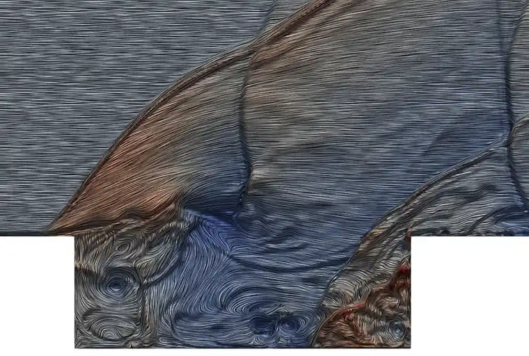
图3将SU2计算的二维超声速空腔流场与试验纹影进行了对比。可以看到计算结果清晰捕捉到了空腔前缘斜激波和各种运动波系结构,计算得到的波系结构形状、相对位置等与试验结果基本一致。

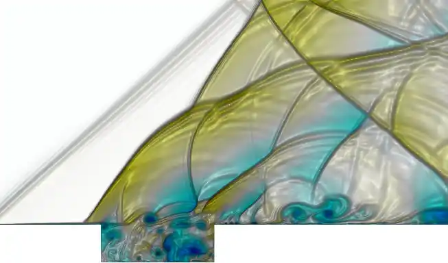
a)


b)图 3 试验纹影结果与计算结果对比
a)
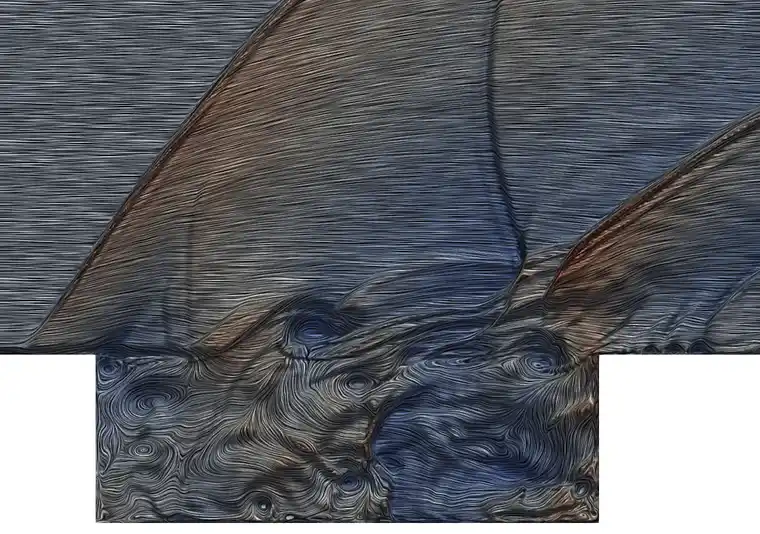
b)图 4 超声速空腔内部流动结构
图4展示了SU2计算得到的超声速空腔内部流动结构。可以清晰看到空腔内部各种尺度的旋涡结构以及运动激波,以及各种流动结构之间的相互作用过程。
采用SU2计算了二维超声速空腔流场,计算得到的波系结构与试验纹影结果符合一致,表明SU2具备模拟二维空腔等超声速非定常流场的能力。
免责声明:本文系网络转载或改编,未找到原创作者,版权归原作者所有。如涉及版权,请联系删
武汉格发信息技术有限公司,格发许可优化管理系统可以帮你评估贵公司软件许可的真实需求,再低成本合规性管理软件许可,帮助贵司提高软件投资回报率,为软件采购、使用提供科学决策依据。支持的软件有: CAD,CAE,PDM,PLM,Catia,Ugnx, AutoCAD, Pro/E, Solidworks ,Hyperworks, Protel,CAXA,OpenWorks LandMark,MATLAB,Enovia,Winchill,TeamCenter,MathCAD,Ansys, Abaqus,ls-dyna, Fluent, MSC,Bentley,License,UG,ug,catia,Dassault Systèmes,AutoDesk,Altair,autocad,PTC,SolidWorks,Ansys,Siemens PLM Software,Paradigm,Mathworks,Borland,AVEVA,ESRI,hP,Solibri,Progman,Leica,Cadence,IBM,SIMULIA,Citrix,Sybase,Schlumberger,MSC Products...