


一、 基本介绍
deeptools是基于Python开发的一套工具,用于处理诸如RNA-seq、ChIP-seq、MNase-seq、ATAC-seq等高通量数据。工具分为四个模块:BAM和bigWig文件处理、质量控制、热图和其他描述性作图、其他。当然也可以简单分为两个部分:数据处理和可视化。
deeptools三大功能:
- Tools for QC
- BAM & bigWig file processing
- Heatmap and summary plot
deeptools常用函数:
- 多样本质控:multiBamSummary (bins/BED-file) → plotCorrelation、plotPCA
- bam转换为bw:bamCoverage、bamCompare → IGV
- reads在基因特征的分布:computeMatrix (scale-regions/reference-point) → plotHeatmap、plotProfile
对于deeptools里的任意子命令,都支持:--help查看帮助文档;--numberOfProcessors/-p设置多核处理;--region/-r CHR:START:END处理部分区域。还有一些过滤用参数部分子命令可用,如ignoreDuplicates去除重复序列,针对匹配到同一方向同一起点的序列,只保留一个(deeptools是在scaling data做低质量数据去除和去重,所以如果数据质量较差及重复数据很多,尽量事先使用samtools进行提前处理);minMappingQuality匹配得分阈值设定;samFlagInclude;samFlagExclue。
二、 使用方法
(1) 多样本质控
多样本分析主要分析处理组不同重复间的相关程度,会用到multiBamSummary、plotCorrelation和plotPCA三个模块。主要目的是看对照组和处理组中的组间差异和组内相似性。如果上一步把BAM转换成BW,那么multiBamSummary可以用multiBigWigSummary替代。
※ multiBamSummary可以用来处理bam文件在基因组上覆盖情况,默认输出npz文件(输出是压缩的numpy数组),衔接 plotCorrelation和 plotPCA进行作图。 有两种模式, bins和 BED-file。bins是给定bin size在全基因组范围内进行coverage的统计,bed-file模式则是给定region进行coverage的统计。Bins模式对相同大小(默认10 kb)的连续bins进行coverage计算,此模式对于评估BAM文件的全基因组相似性非常有用,可以调整bins大小和bins之间的距离。bed-file模式需要用户提供一个BED文件,该文件包含coverage分析应该考虑的所有区域,一个常见的用途是比较一组峰区域的两个不同样品之间的ChIP-seq覆盖率。
# bin mode:
multiBamSummary bins  --bamfiles file1.bam file2.bam  -out results.npz
# BED-file mode:
multiBamSummary BED-file  --BED selection.bed  --bamfiles file1.bam file2.bam  -out results.npz

# example:
multiBamSummary bins  --bamfiles testFiles/*bam  --labels H3K27me3 H3K4me1 H3K4me3 HeK9me3 input  -out readCounts.npz  --outRawCounts readCounts.tab  --minMappingQuality 30  --region 19
# readCounts.tab
chr  start  end   H3K27me3  H3K4me1  H3K4me3  HeK9me3  input
19  10000   20000   0.0     0.0     0.0     0.0     0.0
multiBamSummary bins  --bamfiles chip_rep1_1_sorted.bam chip_rep1_2_sorted.bam chip_rep1_3_sorted.bam chip_rep2_1_sorted.bam ctrl_rep1_1_sorted.bam ctrl_rep1_2_sorted.bam ctrl_rep2_1_sorted.bam  --extendReads 130  -bs 1000  -out results.npz
--bamfiles/-b:用空格分隔不同的bam文件。
--lables/-l:例子:--lables H3k27me3 H3K4me1。
--outFileName/-o/-out:输出文件,输出文件直接可用于plotCorrelation 和plotPCA。
--outRawCounts: 以制表符形式输出每个样本在每个区域的counts数目。
--binSize/-bs:窗口长度,默认为10 kb。
--distanceBetweenBins/-n:默认情况下,multiBamSummary考虑指定binSize的连续bin。然而,为了减少计算时间,可以给定bins之间更大的距离。距离越大,考虑的bins越少。默认值为0。
--region/-r:指定一个染色体的区域,CHR:START:END,例如chr10:456700:891000。
-p:线程数。
--extendReads:延长reads的长度,这个参数不建议RNA-seq添加(由于剪接)。
--ignoreDuplicates:去除PCR重复,依据方向和序列是否完全一致。
--centerReads:reads的mapping会更中心化,利于获得更富集的信号。
--minFragmentLength:过滤ATAC-seq 较短的序列。
-v:设定是否输出信息。
※ Tools for QC:plotCorrelation,plotPCA,plotFingerprint,bamPEFragmentSize,computeGCBias,plotCoverage。都是运用 multiBamSummary得到npz文件统计样本间的相关系数作图和PCA分析作图。plotCorrelation可选Pearson或Spearman方法用于计算相关系数。结果可以保存为描绘成对相关性的散点图或者聚类热图,其中颜色表示相关系数,并且使用最邻近点算法连接聚类,也可以将值保存为表格。
# 散点图
plotCorrelation  -in results.npz  -o results_scatterplot.png  --corMethod spearman  -p scatterplot
# 热图
plotCorrelation  -in results.npz  -o results_heatmap.png  --corMethod spearman  -p heatmap
# 主成分分析
plotPCA  -in results.npz  -o results_pca.png
-in/--corData:绘制图形的Coverage file。
-o/--plotFile:保存的图形文件,文件扩展名决定了格式,可用格式有png、eps、pdf和svg。
-c/--corMethod:计算相关性的方法,spearman或pearson。
-p/--whatToPlot:选择画heatmap还是pairwise scatter plots。
--labels sample1 sample2/-l:自定义标签。
--plotTitle/-T:标题。
Heatmap options:--plotHeight,--plotWidth,--zMin,--zMax,--colorMap
Scatter plot options:--xRange,--yRange,--log1p
plotPCA:--plotHeight,--plotWidth,--PCs,--log2,--colors,--markers
--outFileCorMatrix:[对于plotCorrelation] Save matrix with pairwise correlation values to a tab-separated file.
--outFileNameData:[对于plotPCA,从multiBigwigSummary输出绘图。默认情况下,By default, the loadings for each sample in each principal component is plotted。如果数据被转置,the projections of each sample on the requested principal components is plotted instead。]保存绘图基础数据的文件名,如myPCA.tab。For untransposed data, this is the loading per-sample and PC as well as the eigenvalues. For transposed data, this is the rotation per-sample and PC and the eigenvalues.
--removeOutliers:如果设置了,counts非常大的bins将被移除。具有异常高的reads counts的bins人为地增加了pearson correlation,因此multiBamSummary试图使用中位绝对偏差(MAD)方法去除异常值,该方法应用200的阈值,仅考虑与中位数的极大偏差。
(2) bam转换为bw
BAM文件是SAM的二进制转换版,bigWig是wiggle的二进制版,存放区间的坐标轴信息和相关计分(score),主要用于在基因组浏览器上查看数据的连续密度图,可用wigToBigWig从wiggle进行转换。bedGraph和wiggle格式是基因组浏览器图形轨展示格式,前者展示稀松型数据,体积较大,后者展示按照分箱的连续性数据,体积较小,但是bigWig代表的信息是稍微有点失真的。
deeptools提供bamCoverage和bamCompare进行格式转换,为了能够比较不同的样本,需要对先将基因组分成等宽分箱(bin),统计每个分箱的read数,最后得到描述性统计值。对于两个样本,描述性统计值可以是两个样本的比率,或是比率的log2值,或者是差值。如果是单个样本,可以用SES方法进行标准化。
※ bamCoverage可以用来将bam file转换成bigwig file,同时可以设定 binSize参数从而获取不同的分辨率。在比较非一批数据的时候,还可以设定数据 normalizeTo1X到某个值(一般是该物种基因长度)从而方便进行比较。单纯的可以当作bigwig转换工具,得到的bw文件就可以送去IGV/Jbrowse进行可视化。
# example
bamCoverage  -b input.bam  -o input.bw
bamCoverage  -b input.bam  -o input.bw  (-of bedgraph -e 170)  -bs 100  -r Chr4:12985884:12997458
bamCoverage  -b input.bam  -o input.bw  --binSize 10  (--extendReads  --normalizeUsing RPGC  --effectiveGenomeSize 2150570000  --ignoreForNormalization chrX)

# example
for i in SRR147656{38..47}
do
    bamCoverage  -p 4  --binSize 10  --normalizeUsing BPM  --exactScaling  --smoothLength 30  --centerReads  --bam ${i}._sorted.bam  -o ${i}.bw
done
--bam/-b : 需要操作的bam文件。
--outFileName/-o:输出文件,bw格式的文件。
--outFileFormat/-of:输出格式,有两种选择:bigwig(默认)、bedgraph。
-bs/--binSize:设置分箱的大小,默认50。
--region/-r CHR:START:END:选取某个区域统计。例如--region chr10或-r chr10:456700:891000。
--filterRNAstrand {forward, reverse}:仅统计指定正链或负链,为链特异文库设定的。
-e/--extendReads:拓展了原来的read长度,RNA-seq不适用。
--centerReads:添加此选项使reads相对于fragment length居中。对于双端数据,reads以片段两端定义的片段长度为中心。对于单端数据,使用给定的片段长度。该选项有助于在富集区域周围获得更清晰的信号。
--blackListFileName:排除的区域,输入bed或者gtf文件。
--numberOfProcessors/-p:使用的线程数。
Read coverage normalization options:
如果为了与其他结果进行比较,还需要进行标准化。bamCoverge 具有多种标准化的方法:
RPKM = Reads Per Kilobase per Million mapped reads.
CPM = Counts Per Million mapped reads, same as CPM in RNA-seq.
BPM = Bins Per Million mapped reads, same as TPM in RNA-seq.
RPGC = reads per genomic content (1x normalization).
--normalizeUsing:Use one of the entered methods to normalize the number of reads per bin. By default, no normalization is performed. 可选项为:RPKM, CPM, BPM, RPGC, None,默认是None。
RPKM (per bin) = number of reads per bin / (number of mapped reads (in millions) * bin length (kb)).
CPM (per bin) = number of reads per bin / number of mapped reads (in millions).
BPM (per bin) = number of reads per bin / sum of all reads per bin (in millions).
RPGC (per bin) = number of reads per bin / scaling factor for 1x average coverage.
None = the default and equivalent to not setting this option at all.
This scaling factor is determined from the sequencing depth: (total number of mapped reads * fragment length) / effective genome size. The scaling factor used is the inverse of the sequencing depth computed for the sample to match the 1x coverage. This option requires --effectiveGenomeSize.
--exactScaling:处理所有reads以确定将在输出中使用的确切数字,而不是基于reads的取样来计算scaling factors。这需要更多的时间来计算,但在被过滤后的alignments很少并集中在一起的情况下,会产生更精确的scaling factors。换句话说,只有当基于区域的取样预计会产生不正确的结果时,才需要这样做。
--ignoreForNormalization:指定哪些染色体不需要经过标准化。例如--ignoreForNormalization chrX chrM。
--effectiveGenomeSize:有效基因组大小是基因组中可作图的部分。基因组的大部分是应该被丢弃的NNNN片段。此处提供了一个值表:http://deeptools.readthedocs.io/en/latest/content/feature/effectiveGenomeSize.html。dm6为142573017。
--smoothLength:通过使用分箱附近的read对分箱进行平滑化。smoothLength定义了一个大于binSize的窗口,用于平均reads数量。例如,如果--binSize设置为20,而--smoothLength设置为60,则对于每个bin,考虑bin及其左右邻居的平均值。任何小于--binSize的值都将被忽略,并且不会应用平滑。
※ bamCompare和bamCoverage类似,只不过需要提供两个样本,并且采用SES方法进行标准化,于是多了--ratio参数。可以用来处理treat组和control组的数据,转换成bigwig文件,给出一个binsize内结合强度的比值(默认log2处理)。即输入2个bam文件(treat 和control),输出富集信号的比值,以bigwig或者bedgraph形式存在。
# example
bamCompare  -b1 treatment.bam  -b2 control.bam  -o log2ratio.bw
-bs/--binSize:设置分箱的大小,默认50。
--scaleFactorsMethod {readCount,SES,None}:比较2个样本的方法。(Default: readCount)
--operation {log2,ratio,subtract,add,mean,reciprocal_ratio,first,second}:默认情况下,输出两个样本的log2 ratio。
(3) reads在基因特征的分布
为了统计全基因组范围的peak在基因特征的分布情况,需要用到computeMatrix计算,用plotHeatmap以热图的方式对覆盖进行可视化,用plotProfile以折线图的方式展示覆盖情况。
※ computeMatrix可以计算每个基因区域的结合得分,生成中间文件用以给plotHeatmap和plotProfiles作图。有两种模式,scale-regions mode和reference-point mode,前者用来查看信号在一个区域内分布,后者查看信号相对于某一个点的分布情况。将所有的区域划分为等长的区间称之为bin,然后计算每个bin内所有位点的测序深度,默认用所有位点测序深度的平均值来代表这个区间。输入 bed和bigwig文件,输出用于画profile和heatmap的中间文件。
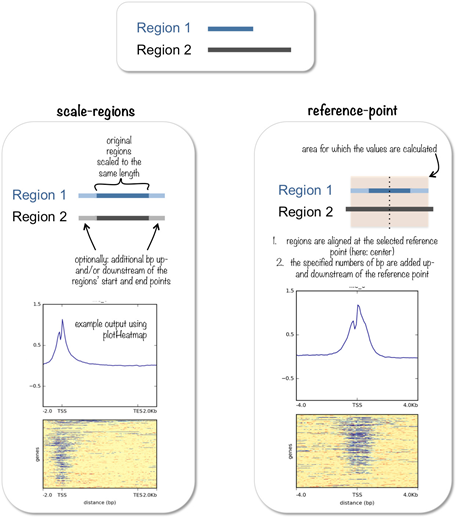
- scale-regions mode简单来说会将给定bed file范围内的结合信号做一个统计(指的是一段长度),并将基因长度统一scale到设定 regionBodyLength的长度,加上统计基因上游和下游Xbp的信号(-b和-a)。-S是提供bigwig文件,-R是提供基因的注释信息。
# example
# computeMatrix scale-regions  -S <biwig file(s)>  -R <bed file>  -b 1000
computeMatrix scale-regions  -p 4  -S test1.bw test2.bw  -R gene19.bed geneX.bed  -b 3000  -a 3000  --regionBodyLength 5000  --skipZeros  -o heatmap.gz  --outFileNameMatrix  matrix.tab  --outFileSortedRegions regions_genes.bed
--scoreFileName/-S:输入的bigwig文件。
--regionsFileName/-R:BED和GTF,包含要绘制的区域。如果给出多个BED文件,则将每个文件视为一组,可以分别绘制。此外,在BED文件中添加一个#符号将使#之前的区域被视为一个组。
--outFileName/-out/-o:gzipped 压缩的矩阵文件,用于plotHeatmap和plotProfile。
--outFileNameMatrix:输出热图的矩阵结果,便于用R语言操作。
--outFileSortedRegions:输出按热图顺序排序好的bed文件结果。
--beforeRegionStartLength/-b:基因上游的碱基长度。(区域文件中定义的区域起点上游的距离。)
--afterRegionStartLength/-a:基因下游的碱基长度。(给定区域终点下游的距离。)
--regionBodyLength/-m:基因body,标准化后的长度。
--skipZeros:跳过全为0的行。
--binSize:默认是10。
-p:线程数。
--startLabel:图中显示的区域开始的标签,默认值为TSS(转录起始位点)。可以改成任何东西,例如peak start,只有在你计划自己绘制结果时有效,plotHeatmap会忽略这个设置。
--endLabel:Default "TES".
--sortRegions {descend,ascend,no,keep}:输出文件是否应该显示已排序的区域。默认情况下不对区域进行排序。只有在你计划自己绘制结果时有效,plotHeatmap会忽略这个设置。未排序的输出将按照处理区域的顺序进行,并且与输入文件中的顺序不匹配。如果要求输出顺序与输入区域的顺序相匹配,那么可以指定keep。(Default: keep)
--averageTypeBins {mean,median,min,max,std,sum}:定义在bin大小范围内使用的统计类型。默认为mean。
--transcriptID:当使用GTF文件提供区域时,只有以此值作为feature的entries(第3列)才会被作为transcripts处理。默认为transcript。
--exonID:当使用GTF文件提供区域时,只有以此值作为feature的entries(第3列)才会被作为exons处理。默认为exon。CDS可能是另一个常见的值。
--transcript_id_designator:每个区域都有一个分配给它的ID。对于BED文件,一般是第4列(name,例如ACTB)。对于GTF文件,一般是一个key:value pair,存储在最后一列中(例如transcript_id "ACTB")。在某些情况下,使用不同的标识符可能很方便,为此,可将其设置为所需的键。
- reference-point mode则是给定一个bed file,以某个点为中心开始统计信号(TSS/TES/center)。
# example
computeMatrix reference-point  --referencePoint TSS  -S H3K4Me3.bw  -R genes.bed  -b 3000  -a 10000  --skipZeros  --binSize 10  -o H3K4me3_TSS.gz  --outFileNameMatrix matrix.tab  --outFileSortedRegions regions_genes.bed
--referencePoint {TSS,TES,center}:reference-point mode专用参数。TSS 为 bed 文件第一个位置,TES 为 bed 文件最后一个位置,center 为 bed 文件中间位置。注意,无论指定了什么,plotHeatmap/plotProfile将默认使用“TSS”作为标签。
在输出的matrix.tab文件中,每一行代表一个转录本,和输入的bed文件中的转录本个数一致,每一列代表bin区间内的平均测序深度,列数的多少和区间的长度以及bin_size有关。在上面这个例子中,选择上下游各3kb的区间,bin大小为10bp,所以总共有3000x2/10, 即600个区间。在可视化时,区间个数越多,画出来的折线图会相对平滑,所以可以适当调整bin的大小,使画出来的图更加美观。
※ plotHeatmap、plotProfile、plotEnrichment,主要用来画热图并包含聚类功能。plotProfile主要用来画密度图,上游数据是 computeMatrix得到的gz file,可以使用 kmean或 hclust聚类。plotHeatmap上游数据也是 computeMatrix得到的gz file。注意:作图会把之前 computeMatrix时候提交的多个bed文件分开作图。如果针对单个bed file进行作图,还可以使用--kmeans参数设定clustering个数。plotHeatmap生成的结果分成了两部分,第一部分和plotProfile的结果相同,第二部分是一个热图,就是将生成的tab文件中的内容绘制了一个热图。
# example
plotProfile  -m matrix.gz  -out profile.pdf  --plotFileFormat pdf   --dpi 720
plotProfile  -m matrix.gz  -out profile.png  --perGroup  --kmeans 2
plotProfile  -m matrix.gz  -out profile.png  --numPlotsPerRow 2  --plotTitle "Test data profile"

# example
plotHeatmap  -m matrix.gz  -o heatmap.pdf  --plotFileFormat pdf  --dpi 720
plotHeatmap  -m matrix.gz  -o heatmap.pdf  --plotFileFormat pdf  --dpi 720  --colorMap RdBu  --whatToShow 'heatmap and colorbar'  --zMin -3  --zMax 3  --kmeans 4
--matrixFile/-m:computeMatrix得到的matrix.gz。
--outFileName/-out/-o:保存图像的文件名。文件结尾将用于确定图像格式。可选格式有:png、ep、pdf、svg。
--outFileSortedRegions:跳过零或最小/最大阈值后保存区域的文件名。文件中区域的顺序遵循选定的排序顺序。这对于在保持第一个热图的排序的同时生成其他热图是有用的。(Example: Heatmap1sortedRegions.bed)
--outFileNameData:File name to save the data underlying data for the average profile, e.g. myProfile.tab.
--dpi:分辨率,默认200。
--perGroup:computeMatrix如果给出多个BED文件,则将每个文件视为一组。默认情况下,按样本绘制所有组(一个样本绘制一个profile plot和heatmap,profile里面有n条线,heatmap上下分为n个部分;如果有m个样本则绘制m列)。使用此选项代替按组绘制所有样本(每个BED文件生成一个profile plot和heatmap,即n列;如果有m个样本,每个profile里面有m条线,heatmap分为上下m个部分)。这仅在有多组区域时有用。
--kmeans:如果设置了此选项,将使用k-means算法将矩阵分成多个clusters。仅适用于未分组的数据,否则只会对第一个组进行聚类。
--hclust:Number of clusters to compute. 如果设置了此选项,则使用ward linkage使用分层聚类算法将矩阵拆分为多个聚类。仅适用于未分组的数据,否则只会对第一个组进行聚类。如果有超过1000个区域,hclust可能会非常慢,在这些情况下,可能更适合kmeans。
--startLabel:[only for scale-regions mode] Label shown in the plot for the start of the region. Default is TSS (transcription start site), but could be changed to anything, e.g. "peak start".
--endLabel:[only for scale-regions mode] Label shown in the plot for the region end. Default is TES (transcription end site).
--refPointLabel:[only for reference-point mode] Label shown in the plot for the reference-point. Default is the same as the reference point selected (e.g. TSS), but could be anything.
--labelRotation:Rotation of the X-axis labels in degrees. The default is 0, positive values denote a counter-clockwise rotation.
--regionsLabel:Labels for the regions plotted in the heatmap. If more than one region is being plotted, a list of labels separated by spaces is required.
--samplesLabel:Labels for the samples plotted. The default is to use the file name of the sample. The sample labels should be separated by spaces and quoted if a label itselfcontains a space E.g. --samplesLabel label-1 "label 2"
--plotTitle:Title of the plot, to be printed on top of the generated image. Leave blank for no title.
--yAxisLabel:Y-axis label for the top panel.
--yMin,--yMax:Minimum/Maximum value for the Y-axis. Multiple values, separated by spaces can be set for each profile. If the number of yMin values is smaller than the number of plots, the values are recycled.
--legendLocation {best,upper-right,upper-left,upper-center,lower-left,lower-right,lower-center,center,center-left,center-right,none}:Location for the legend in the summary plot. Note that "none" does not work for the profiler. (default: best)
plotProfile options:
--averageType {mean,median,min,max,std,sum}:The type of statistic that should be used for the profile.
--plotHeight:Plot height in cm. (default: 7)
--plotWidth:Plot width in cm. The minimum value is 1 cm. (default: 11)
--plotType {lines,fill,se,std,overlapped_lines,heatmap}:"lines" will plot the profile line based on the average type selected. "fill" fills the region between zero and the profile curve. The fill in color is semi transparent to distinguish different profiles. "se" and "std" color the region between the profile and the standard error or standard deviation of the data. As in the case of fill, a semi-transparent color is used. "overlapped_lines" plots each region's value, one on top of the other. "heatmap" plots a summary heatmap. (default: lines)
--colors:用于绘制lines的颜色列表(不适用于--plotType overlapped_lines)。接受颜色名称和html十六进制字符串(例如#eeff22)。颜色名称应该用空格分隔,例如--colors red blue green。
--numPlotsPerRow:Number of plots per row (default: 8)
plotHeatmap options:
--interpolationMethod:如果热图图像包含大量列,通常最好使用interpolation方法来产生更好的结果。默认情况下,如果列数等于或小于1000,plotHeatmap使用nearest方法。否则,使用bilinear方法。可选方法包括:"nearest", "bilinear", "bicubic", "gaussian" (default: auto)。
--plotType {lines,fill,se,std}:"lines" will plot the profile line based on the average type selected. "fill" fills the region between zero and the profile curve. The fill in color is semi transparent to distinguish different profiles. "se" and "std" color the region between the profile and the standard error or standard deviation of the data. (default: lines)
--linesAtTickMarks:Draw dashed lines from all tick marks through the heatmap. This is then similar to the dashed line draw at region bounds when using a reference point and --sortUsing region_length.
--missingDataColor:default: black.
--colorMap:Color map to use for the heatmap. 如果绘制了多个热图,可以单独输入每个热图的颜色(例如--colorMap Reds Blues)。如果color maps的数量小于正在绘制的热图的数量,则color maps将被循环。可选颜色包括:magma、inferno、plasma、viridis、cividis、twilight、twilight_shifted、turbo、Blues、BrBG、BuGn、BuPu、CMRmap、GnBu、Greens、Greys、OrRd、Oranges、PRGn、PiYG、PuBu、PuBuGn、PuOr、PuRd、Purples、RdBu、RdGy、RdPu、RdYlBu、RdYlGn、Reds、Spectral、Wistia、YlGn、YlGnBu、YlOrBr、YlOrRd、afmhot、autumn、binary、bone、brg、bwr、cool、coolwarm、copper、cubehelix、flag、gist_earth、gist_gray、gist_heat、gist_ncar、gist_rainbow、gist_stern、gist_yarg、gnuplot、gnuplot2、gray、hot、hsv、jet、nipy_spectral、ocean、pink、prism、rainbow、seismic、spring、summer、terrain、winter、Accent、Dark2、Paired、Pastel1、Pastel2、Set1、Set2、Set3、tab10、tab20、tab20b、tab20c、rocket、mako、vlag、icefire (default: RdYlBu)
--alpha:The alpha channel (transparency) to use for the heatmaps. The default is 1.0 and values must be between 0 and 1. (default: 1.0)
--colorList:用于创建colormap的颜色列表。例如,如果设置了--colorList black,yellow,blue,则创建了一个以黑色开始,以黄色继续,以蓝色结束的colormap。如果选择了此选项,它将覆盖所选的--colorMap。
--colorNumber:控制了从一种颜色过渡到另一种颜色的数量,默认256。
--zMin:Minimum value for the heatmap intensities.
--zMax:Maximum value for the heatmap intensities.
--heatmapHeight:Plot height in cm. The default for the heatmap height is 28. The minimum value is 3 and the maximum is 100.
--heatmapWidth:Plot width in cm. The default value is 4. The minimum value is 1 and the maximum is 100.
--whatToShow:default: plot, heatmap and colorbar. Other options are: "plot and heatmap", "heatmap only", "heatmap and colorbar".
--boxAroundHeatmaps: By default black boxes are plot around heatmaps. This can be turned off by setting --boxAroundHeatmaps no (default: yes)
--xAxisLabel: Description for the x-axis label. (default: gene distance (bp))

 技术文档
技术文档
 推荐好文
推荐好文


 155-2731-8020