


软件

产品


本文将从iris数据集创建一个线性分类器。如前所述,用花萼宽度和花萼长度的特征可以创建一个线性二值分类器来预测是否为山鸢尾花。
# Linear Support Vector Machine: Soft Margin# ----------------------------------
## This function shows how to use TensorFlow to# create a soft margin SVM#
# We will use the iris data, specifically:#  x1 = Sepal Length
#  x2 = Petal Width# Class 1 : I. setosa# Class -1: not I. setosa
## We know here that x and y are linearly seperable
# for I. setosa classification.import matplotlib.pyplot as pltimport numpy as npimport tensorflow as
tffrom sklearn import datasetsfrom tensorflow.python.framework import opsops.reset_default_graph()
# 创建一个计算图会话sess = tf.Session()# 加载需要的数据集# 加载iris数据集的第一列和第四列特征变量,其为花萼长度和花萼宽度。
# 加载目标变量时,山鸢尾花为1,否则为-1
# iris.data = [(Sepal Length, Sepal Width, Petal Length,
Petal Width)]iris = datasets.load_iris()x_vals = np.array([[x[0],
x[3]] for x in iris.data])y_vals = np.array([1 if y == 0 else -1 for y in iris.target])
# 分割数据集为训练集和测试集train_indices = np.random.choice(len(x_vals),
round(len(x_vals)*0.8),
replace=False)test_indices = np.array(list(set(range(len(x_vals)))
- set(train_indices)))x_vals_train = x_vals[train_indices]x_vals_test
 = x_vals[test_indices]y_vals_train = y_vals[train_indices]y_vals_test = y_vals[test_indices]
 # 分割数据集为训练集和测试集batch_size = 100# 初始化占位符x_data = tf.placeholder(shape=[None, 2],
 dtype=tf.float32)y_target = tf.placeholder(shape=[None, 1], dtype=tf.float32)
 # Create variables for linear regression# 模型变量# 对于这个支持向量机算法,我们希望用非常大的批量大小来帮助其收敛。
 # 可以想象一下,非常小的批量大小会使得最大间隔线缓慢跳动。# 在理想情况下,也应该缓慢减小学习率,但是这已经足够了。
 # A变量的形状是2×1,因为有花萼长度和花萼宽度两个变量A = tf.Variable(tf.random_normal(shape=[2, 1]))b = tf
 .Variable(tf.random_normal(shape=[1, 1]))# Declare model operations
 # 声明模型输出# 对于正确分类的数据点,如果数据点是山鸢尾花,则返回的数值大于或者等于1;
 # 否则返回的数值小于或者等于-1model_output = tf.subtract(tf.matmul(x_data, A), b)
 # Declare vector L2 'norm' function squared# 声明最大间隔损失函数# 我们将声明一个函数来计算向量的L2范数。
 # 接着增加间隔参数α。# 声明分类器损失函数,并把前面两项加在一起l2_norm = tf.reduce_sum(tf.square(A))
 # Declare loss function# Loss = max(0, 1-pred*actual) + alpha * L2_norm(A)^2
 # L2 regularization parameter, alphaalpha = tf.constant([0.01])
 # Margin term in lossclassification_term = tf.reduce_mean(tf.maximum(0., tf
 .subtract(1., tf.multiply(model_output, y_target))))# Put terms togetherloss = tf
 .add(classification_term, tf.multiply(alpha, l2_norm))# Declare prediction function
 # 声明预测函数和准确度函数prediction = tf.sign(model_output)accuracy = tf.reduce_mean(tf.cast(tf
 .equal(prediction, y_target), tf.float32))# Declare optimizer# 声明优化器函数my_opt = tf.train
 .GradientDescentOptimizer(0.01)train_step = my_opt.minimize(loss)# 初始化模型变量init = tf
 .global_variables_initializer()sess.run(init)
 # Training looploss_vec = []train_accuracy = []test_accuracy = []for i in range(500):
 rand_index = np.random.choice(len(x_vals_train), size=batch_size)
 rand_x = x_vals_train[rand_index]    rand_y = np.transpose([y_vals_train[rand_index]])
 sess.run(train_step, feed_dict={x_data: rand_x, y_target: rand_y})
 temp_loss = sess.run(loss, feed_dict={x_data: rand_x, y_target: rand_y})
 loss_vec.append(temp_loss)    train_acc_temp = sess.run(accuracy, feed_dict={
 x_data: x_vals_train,        y_target: np.transpose([y_vals_train])})    train_accuracy
 .append(train_acc_temp)    test_acc_temp = sess.run(accuracy, feed_dict={
 x_data: x_vals_test,        y_target: np.transpose([y_vals_test])})    test_accuracy
 .append(test_acc_temp)    if (i + 1) % 100 == 0:        print('Step #{} A = {}, b = {}'
 .format(            str(i+1),            str(sess.run(A)),            str(sess.run(b))        ))
 print('Loss = ' + str(temp_loss))# 抽取系数# 分割x_vals为山鸢尾花(I.setosa)和非山鸢尾花(non-I.setosa)[[a1],
 [a2]] = sess.run(A)[[b]] = sess.run(b)slope = -a2/a1y_intercept = b/a1
 # Extract x1 and x2 valsx1_vals = [d[1] for d in x_vals]# Get best fit linebest_fit = []for i in x1_vals:
 best_fit.append(slope*i+y_intercept)# Separate I.
 setosasetosa_x = [d[1] for i, d in enumerate(x_vals) if y_vals[i] == 1]setosa_y = [d[0] for i,
 d in enumerate(x_vals) if y_vals[i] == 1]not_setosa_x = [d[1] for i,
 d in enumerate(x_vals) if y_vals[i] == -1]not_setosa_y = [d[0] for i,
 d in enumerate(x_vals) if y_vals[i] == -1]# Plot data and lineplt.plot(setosa_x, setosa_y,
 'o', label='I. setosa')plt.plot(not_setosa_x, not_setosa_y, 'x',
 label='Non-setosa')plt.plot(x1_vals, best_fit, 'r-', label='Linear Separator',
  linewidth=3)plt.ylim([0, 10])plt.legend(loc='lower right')plt.title('Sepal Length vs Pedal Width')plt
  .xlabel('Pedal Width')plt.ylabel('Sepal Length')plt.show()# Plot train/test accuraciesplt
  .plot(train_accuracy, 'k-', label='Training Accuracy')plt.plot(test_accuracy, 'r--',
   label='Test Accuracy')plt.title('Train and Test Set Accuracies')plt.xlabel('Generation')plt
   .ylabel('Accuracy')plt.legend(loc='lower right')plt.show()# Plot loss over timeplt
   .plot(loss_vec, 'k-')plt.title('Loss per Generation')plt.xlabel('Generation')plt
   .ylabel('Loss')plt.show()1.2.3.4.5.6.7.8.9.10.11.12.13.14.15.16.17.18.19.20.21.22.23.24.25.26
   .27.28.29.30.31.32.33.34.35.36.37.38.39.40.41.42.43.44.45.46.47.48.49.50.51.52.53.54.55.56.57.
   58.59.60.61.62.63.64.65.66.67.68.69.70.71.72.73.74.75.76.77.78.79.80.81.82.83.84.85.86.87.88.
   89.90.91.92.93.94.95.96.97.98.99.100.101.102.103.104.105.106.107.108.109.110.111.112.113.114.
   115.116.117.118.119.120.121.122.123.124.125.126.127.128.129.130.131.132.133.134.135.136.137.
   138.139.140.141.142.143.144.145.146.147.148.149.150.151.152.153.154.155.156.157.158.159.160.
   161.162.163.164.165.166.167.168.169.170.171.172.173.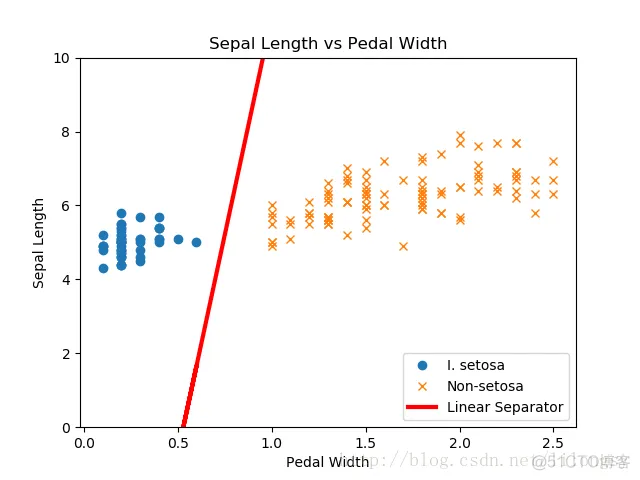
线性支持向量机拟合
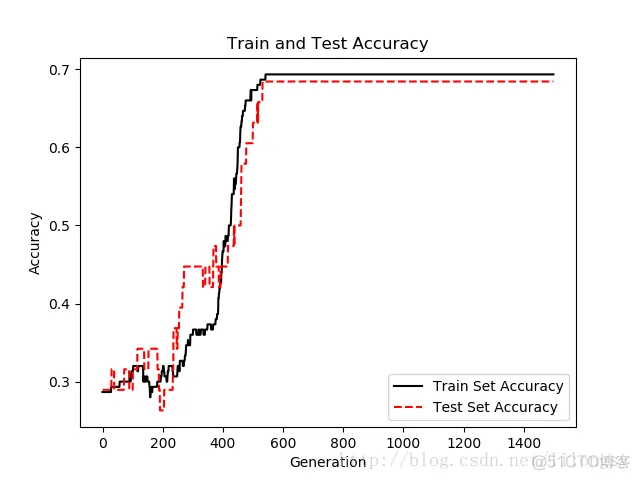
训练集和测试集迭代的准确度。由于两类目标是线性可分的,得到准确度是100%从图中可以看出,训练集和测试集迭代训练。由于两类目标是线性可分的,我们得到准确度是100%。
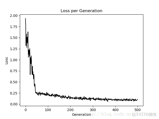
迭代500次的最大间隔图
免责声明:本文系网络转载或改编,未找到原创作者,版权归原作者所有。如涉及版权,请联系删
武汉格发信息技术有限公司,格发许可优化管理系统可以帮你评估贵公司软件许可的真实需求,再低成本合规性管理软件许可,帮助贵司提高软件投资回报率,为软件采购、使用提供科学决策依据。支持的软件有: CAD,CAE,PDM,PLM,Catia,Ugnx, AutoCAD, Pro/E, Solidworks 等。
 技术文档
技术文档
 推荐好文
推荐好文


 155-2731-8020


